Module 7: Unsupervised learning 30 min5 min quick readClassical ML
DBSCAN, hierarchical clustering, and Gaussian mixtures
Choose a clustering method by the shape and density of your clusters, run DBSCAN by hand, read a dendrogram, and use soft memberships and anomaly scores.
Before this: K-means clustering
Quick read: the intuition, interactive visualization, summary, and interview questions. The math, implementation, engineering, and knowledge-check sections are hidden.
Mental model. K-means asks "which center is nearest?" DBSCAN asks "is this point in a crowded neighborhood?" Hierarchical clustering asks "which groups should merge next?" A Gaussian mixture asks "how likely is this point under each of several bell curves?" Different questions find different structure.
You will learn to
- Classify points as core, border, or noise in DBSCAN and tune ε and min_samples.
- Build and cut a dendrogram from hierarchical clustering.
- Explain Gaussian mixture models, soft memberships, and the EM idea.
- Use clustering ideas for anomaly detection.
- Pick a method from the data's cluster shapes, sizes, and noise.
Why it matters. K-means fails on curved shapes, unequal sizes, and outliers, which are common in real data. These three methods cover most of what K-means can't, and density ideas power practical anomaly detection.
1. Intuition
DBSCAN (density-based). A point is core if at least min_samples points (including itself) lie within distance ε. Clusters grow by chaining core points that are within ε of each other, then adding border points that are near a core point. Everything else is noise. You never choose K, and clusters can be any shape.
Hierarchical (agglomerative). Start with every point as its own cluster and repeatedly merge the two closest clusters. The full merge history is a tree, the dendrogram. Cut it at a height to get a clustering; different heights give coarser or finer groups.
Gaussian mixture model (GMM). Assume the data comes from K overlapping bell-shaped (Gaussian) clouds, each with its own center, spread, and orientation. Each point gets a probability of belonging to each cloud: soft membership. A point between two clusters might be 60/40.
2. Visualization
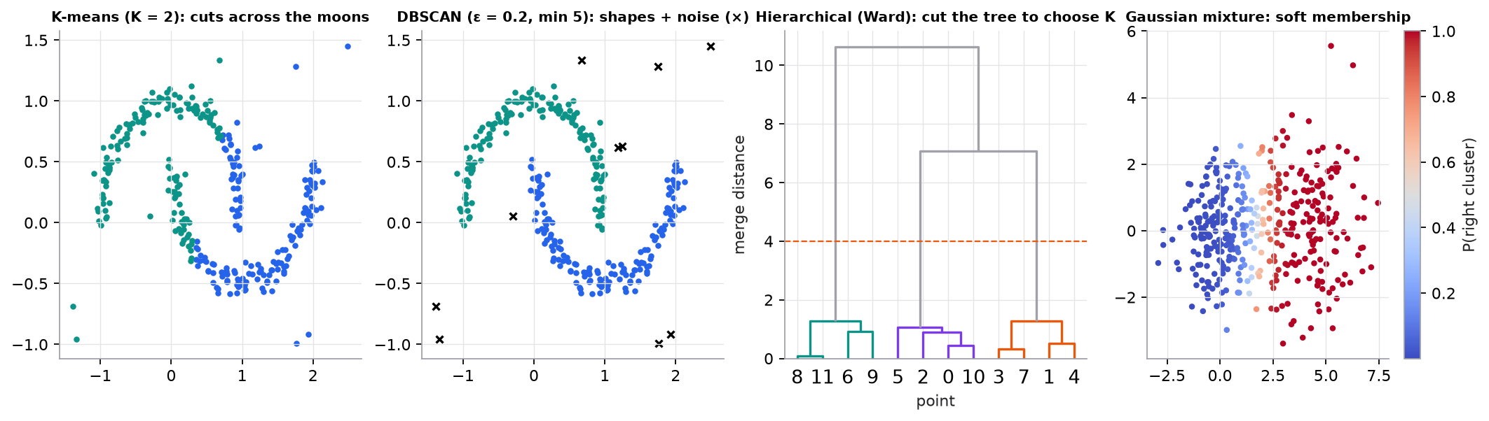
Synthetic data. On two moons plus 15 random points, DBSCAN finds both moons and labels 10 points as noise; K-means can only draw a straight boundary.
Interactive: the K-means lab's "Rings" and "Stretched" presets show the shapes that motivate these methods. Open it.
3. The math
Symbols
| Symbol | Meaning |
|---|---|
| ε | DBSCAN neighborhood radius |
min_samples | points (including itself) needed within ε for a core point |
| mixing weight of component (sums to 1) | |
| mean and covariance of Gaussian component | |
| responsibility: probability point belongs to component |
Gaussian mixture
Expectation-maximization (EM) alternates: compute responsibilities (E-step), then re-estimate as responsibility-weighted averages (M-step). K-means is the limiting case with hard assignments and identical round clusters.
Linkage for hierarchical clustering
The distance between clusters and can be the closest pair (single linkage, finds chains), the farthest pair (complete), the average pair (average), or the increase in within-cluster variance from merging (Ward, which produces compact clusters similar to K-means).
Worked example: DBSCAN by hand
Points on a line: , with ε = 0.6 and min_samples = 3.
| Point | Neighbors within 0.6 (including itself) | Count | Type |
|---|---|---|---|
| 1.0 | 1.0, 1.5 | 2 | border (near core 1.5) |
| 1.5 | 1.0, 1.5, 2.0 | 3 | core |
| 2.0 | 1.5, 2.0, 2.4 | 3 | core |
| 2.4 | 2.0, 2.4 | 2 | border (near core 2.0) |
| 6.0 | 6.0, 6.3 | 2 | border (near core 6.3) |
| 6.3 | 6.0, 6.3, 6.8 | 3 | core |
| 6.8 | 6.3, 6.8 | 2 | border |
| 12.0 | 12.0 | 1 | noise |
Result: cluster 0 = {1.0, 1.5, 2.0, 2.4}, cluster 1 = {6.0, 6.3, 6.8}, and 12.0 is noise. scikit-learn returns exactly these labels.
Worked example: soft membership
A two-component GMM fit to synthetic data (a tight cluster at 0 and a wider one at 4) gives the point responsibilities . Although it is closer to the left center, the right cluster's larger spread makes the point more plausible under it. K-means would assign it to the left cluster with full confidence.
4. Implementation
Build it from scratch
DBSCAN and the EM loop for a Gaussian mixture each fit in about 20 lines of NumPy. The full script, which checks both against scikit-learn, is code/07-unsupervised/clustering.py.
DBSCAN, part 1: neighbors and core points. Compute all pairwise distances once, list each point's ε-neighbors (including itself, as in the worked example), and mark a point core when it has at least min_samples of them.
def dbscan(X, eps, min_samples):
    """Label each point with a cluster id, or -1 for noise. Also return the core-point mask."""
    D = np.sqrt(((X[:, None, :] - X[None, :, :]) ** 2).sum(axis=2))   # [n, n] pairwise distances
    nbrs = [np.flatnonzero(row <= eps) for row in D]                 # neighbors, including itself
    core = np.array([len(nb) >= min_samples for nb in nbrs])
    labels = np.full(len(X), -1)
    cluster = 0
Predict: on the line example with ε = 0.6, how many entries does nbrs hold for the point 12.0, and is it core?
DBSCAN, part 2: grow clusters. Start a new cluster at each unlabeled core point and flood-fill: every neighbor joins, but only core neighbors are pushed on the stack to expand further. Border points join a cluster and stop there; whatever is never reached keeps the label −1 (noise).
    for i in np.flatnonzero(core):
        if labels[i] != -1:                                          # already reached from another core point
            continue
        labels[i], stack = cluster, [i]
        while stack:                                                 # flood-fill through core points
            j = stack.pop()
            for q in nbrs[j]:
                if labels[q] == -1:
                    labels[q] = cluster                              # core or border point joins
                    if core[q]:
                        stack.append(q)                              # only core points keep expanding
        cluster += 1
    return labels, core
Predict: if you removed the if core[q] check and pushed every neighbor, what would happen to 1.0 and 2.4 in the worked example, and to the two moons when a few noise points sit between them?
Gaussian density. EM needs for every point. The einsum computes row by row (the squared Mahalanobis distance), so an elongated covariance makes distance along the long axis cheap.
def gauss_pdf(X, mean, cov):
    """Multivariate normal density N(x | mean, cov) for every row of X."""
    d = X - mean                                                     # [n, p]
    q = np.einsum("ij,jk,ik->i", d, np.linalg.inv(cov), d)           # squared Mahalanobis distance
    return np.exp(-0.5 * q) / np.sqrt((2 * np.pi) ** X.shape[1] * np.linalg.det(cov))
Predict: with cov the identity matrix, what does q reduce to?
EM loop. The E-step turns weighted densities into responsibilities (rows of R, each summing to 1). The M-step is K-means' update step with soft weights: effective points, new weights, weighted means, weighted covariances. The tiny ridge 1e-6 * I keeps a component from collapsing onto a single point.
def gmm_em(X, k, iters=200, seed=0, tol=1e-8):
    """Fit a full-covariance Gaussian mixture with EM. Returns weights, means, covariances, responsibilities."""
    n, p = X.shape
    r = np.random.default_rng(seed)
    pi, mu = np.full(k, 1 / k), X[r.choice(n, k, replace=False)]    # equal weights, random points as means
    S = np.array([np.cov(X.T) for _ in range(k)])                    # start every component at the data covariance
    prev = -np.inf
    for _ in range(iters):
        dens = np.stack([pi[j] * gauss_pdf(X, mu[j], S[j]) for j in range(k)], axis=1)   # [n, k]
        ll = np.log(dens.sum(axis=1)).sum()                          # log-likelihood never decreases
        R = dens / dens.sum(axis=1, keepdims=True)                   # E-step: responsibilities, rows sum to 1
        Nk = R.sum(axis=0)                                           # M-step: effective points per component
        pi, mu = Nk / n, (R.T @ X) / Nk[:, None]
        S = np.array([(R[:, j, None] * (X - mu[j])).T @ (X - mu[j]) / Nk[j] + 1e-6 * np.eye(p)
                      for j in range(k)])                            # small ridge stops collapse onto one point
        if ll - prev < tol:
            break
        prev = ll
    return pi, mu, S, R, ll
Predict: if you replaced each row of R with a one-hot vector at its largest entry fixed every S[j] to the identity, and kept every weight at 1/k, which algorithm would this loop become?
Hierarchical clustering has no from-scratch version here: the naive algorithm (recompute all cluster distances after every merge) is , and SciPy's linkage is the standard tool.
Use the library
In production, use scikit-learn for DBSCAN and Gaussian mixtures and SciPy for the dendrogram. Scale first, because every method here uses distances.
from scipy.cluster.hierarchy import dendrogram, fcluster, linkage
from sklearn.cluster import DBSCAN
from sklearn.mixture import GaussianMixture
from sklearn.neighbors import NearestNeighbors
from sklearn.preprocessing import StandardScaler

X = StandardScaler().fit_transform(X_raw)

# DBSCAN: pick eps from the "knee" of sorted k-th neighbor distances
dists, _ = NearestNeighbors(n_neighbors=5).fit(X).kneighbors(X)
labels = DBSCAN(eps=0.3, min_samples=5).fit_predict(X)      # -1 marks noise

Z = linkage(X, method="ward")
labels_h = fcluster(Z, t=3, criterion="maxclust")            # cut into 3 clusters

gmm = GaussianMixture(n_components=3, covariance_type="full", random_state=0).fit(X)
probs = gmm.predict_proba(X)                                  # soft memberships
anomaly_score = -gmm.score_samples(X)                         # low likelihood = unusual
GaussianMixture stops when the average per-point log-likelihood improves by less than tol, which defaults to 1e-3. On the two-blob example that stops after 3 iterations, with instead of the converged 0.240. Check gmm.converged_ and gmm.n_iter_, and lower tol when you read individual probabilities.
Run it
From guide/:
uv run code/07-unsupervised/clustering.pyKey lines of output:
DBSCAN eps=0.6 min_samples=3
  from scratch labels: [0, 0, 0, 0, 1, 1, 1, -1]  core: [1, 2, 5]
  scikit-learn labels: [0, 0, 0, 0, 1, 1, 1, -1]  core: [1, 2, 5]
GMM on two synthetic blobs (tight at x=0, wide at x=4)
  from scratch: weights [0.499 0.501], means x [0.003 3.879], log-likelihood -1524.10
  scikit-learn: weights [0.499 0.501], means x [0.004 3.88 ], log-likelihood -1524.10
  P(cluster | x=(2.2, 0)): from scratch [0.24 0.76], scikit-learn [0.24 0.76] (left, right)
moons: DBSCAN found 2 clusters and 10 noise points; from scratch agrees on every point: True
The DBSCAN labels match the table in the worked example: indices 1, 2, and 5 (the points 1.5, 2.0, 6.3) are core, and 12.0 is noise. EM from scratch reaches the same likelihood and the same soft membership as scikit-learn.
5. Engineering
| Method | Strength | Weakness |
|---|---|---|
| K-means | fast, simple, scales to millions | round, similar-size clusters; must pick K; outlier-sensitive |
| DBSCAN | arbitrary shapes, labels noise, no K | sensitive to ε and scaling; struggles with varying densities (HDBSCAN helps) |
| Hierarchical | nested structure, dendrogram for exploration | memory, slow beyond tens of thousands of points |
| Gaussian mixture | soft memberships, elliptical clusters, likelihoods | assumes Gaussian shapes; initialization matters; choose K (BIC helps) |
Anomaly detection. Points DBSCAN labels as noise, points with low GMM likelihood, or points far from their K-means centroid are candidate anomalies. Isolation Forest is another common, scalable choice. Anomaly scores need a threshold, and that threshold should be set with whatever labeled incidents you have.
Choosing K for GMMs. Use BIC or AIC (they penalize extra components) together with domain review.
Watch outFailure modes. Unscaled features changing every distance; one ε that can't fit clusters of different densities; reading dendrogram structure in random data; GMM components collapsing onto single points (use regularization or a different covariance type).
Common mistakes
- Running DBSCAN with default ε on unscaled data.
- Treating DBSCAN noise as errors to delete rather than signals to inspect.
- Using hierarchical clustering on 1 million points.
- Reading GMM probabilities from a fit that stopped early: check
converged_and lowertol.
6. Knowledge check
Quiz: DBSCAN, hierarchical clustering, and Gaussian mixtures
DBSCAN with ε = 1 and min_samples = 3. Point P has two other points within distance 1. What is P?
Practice exercise. With the same points and ε = 0.6, what changes if min_samples = 2?
Solution
Every point with at least one neighbor within 0.6 becomes core: 1.0, 1.5, 2.0, 2.4, 6.0, 6.3, 6.8. The clusters stay {1.0–2.4} and {6.0–6.8}, but now all of their points are core. 12.0 is still noise (only itself).
Implementation challenge. Generate three blobs with very different densities. Show that one DBSCAN ε can't separate all three well, then try HDBSCAN (sklearn.cluster.HDBSCAN) and compare.
Summary
- DBSCAN grows clusters from dense core points, finds arbitrary shapes, and labels noise; tune ε and
min_samples, and scale first. - Hierarchical clustering builds a merge tree; cut the dendrogram to choose the number of clusters.
- Gaussian mixtures give soft memberships and likelihoods via EM; K-means is a hard, round special case.
- Low density or low likelihood points are natural anomaly candidates.
Next: PCA, t-SNE, and UMAP
Related: K-means · Model card: DBSCAN · Model card: Gaussian mixture
Interview angle
Explain DBSCAN. When would you choose it over K-means?
DBSCAN defines clusters as dense regions. A point is a core point if at least min_samples points (including itself) lie within radius ε. Clusters form by connecting core points within ε of each other, plus border points within ε of a core point; everything else is labeled noise. Choose it over K-means when clusters have arbitrary, non-convex shapes (rings, curved bands), when you don't know the number of clusters, and when outliers exist and should be flagged rather than forced into a cluster. Downsides: one ε can't fit clusters of very different densities (HDBSCAN handles that), results are sensitive to scaling and to ε, and it struggles in high dimensions where distances concentrate. To pick ε, sort every point's distance to its min_samples-th nearest neighbor, plot the curve, and look for the knee.
How does a Gaussian mixture model differ from K-means, and what is EM doing?
A GMM models the data as : each component has its own mean, its own covariance (so elliptical shapes and different spreads), and a mixing weight. EM alternates two steps. The E-step computes responsibilities , the posterior probability that point came from component , via Bayes' rule. The M-step re-estimates each , , and as responsibility-weighted averages. Each iteration never decreases the likelihood, and like K-means, it converges to a local optimum; K-means is the limit with hard assignments and identical round clusters. Practical differences: soft membership (the lesson's point at is 76% the wider cluster despite being nearer the tight one), a likelihood for anomaly scoring, and BIC for choosing . Costs: parameters per full covariance, and components can collapse onto single points without regularization.
DBSCAN labels 90% of your points as noise on one run and merges everything into one cluster on another. What do you adjust?
Both point to ε being wrong for the data's scale. Mostly noise: ε is too small, or min_samples too large, relative to typical neighbor distances, so few points qualify as core. One giant cluster: ε is large enough that dense regions connect through bridges of sparse points. Steps: first standardize the features, since an unscaled feature dominates every distance and makes any single ε wrong. Then compute each point's distance to its -th nearest neighbor with = min_samples, sort, plot, and set ε near the knee where distances start rising sharply. A common starting point for min_samples is about twice the number of features, larger for noisy data. If clusters genuinely differ in density, no single ε works: switch to HDBSCAN, which effectively scans across ε and keeps the most stable clusters. In high dimensions, reduce dimensionality first.
When would you use hierarchical clustering, and why not on a million points?
Agglomerative clustering starts with every point as its own cluster and repeatedly merges the closest pair, producing a dendrogram that shows structure at every scale; cutting it at different heights gives different numbers of clusters without refitting. Use it for exploration on small-to-medium data, when nested structure is meaningful (product taxonomies, gene families), or when you need a custom distance. Linkage matters: single linkage chains through bridges, complete and average linkage make compact groups, and Ward behaves like K-means. It doesn't scale: standard implementations need the pairwise distance matrix, memory. For points that's about distances even storing only half the symmetric matrix, roughly 2 TB in float32, and time is to . For large data, cluster a sample, or form a few thousand mini-batch K-means micro-clusters and run hierarchical clustering on their centroids.