Module 0: Mathematical and programming foundations 35 min6 min quick readMathematics
Probability and statistics
Conditional probability, Bayes' rule, expectation, variance, common distributions, sampling, and why correlation is not causation.
Quick read: the intuition, interactive visualization, summary, and interview questions. The math, implementation, engineering, and knowledge-check sections are hidden.
Mental model. Probability is bookkeeping for uncertainty. A model's output is usually a probability, its loss is usually a log-probability, and its evaluation is a statistical estimate from a finite sample.
You will learn to
- Compute joint, marginal, and conditional probabilities.
- Apply Bayes' rule, including the base-rate effect that surprises almost everyone.
- Compute expectation and variance, and recognize normal, Bernoulli, binomial, and categorical distributions.
- Explain sampling error and why a metric from a test set is an estimate.
- Separate correlation from causation with a concrete example.
Why it matters. Logistic regression outputs . Cross-entropy is a negative log-probability. Naive Bayes is Bayes' rule. Language models output a categorical distribution over tokens. And every evaluation number you report is a sample statistic with uncertainty.
1. Intuition
Conditional probability is probability after you learn something. The chance a random email is spam might be 20%; the chance it is spam given that it contains "free money" is much higher.
Bayes' rule flips a conditional: from "how often does a positive test happen when someone is sick" to "how likely is someone sick given a positive test." The second depends heavily on how common the disease is in the first place (the base rate). A 95%-accurate test for a rare disease produces mostly false alarms.
Expectation is the long-run average; variance measures spread around it.
Correlation means two quantities move together. It does not tell you that one causes the other: ice-cream sales and swimming incidents both rise in summer because of temperature, not because of each other.
2. Visualization
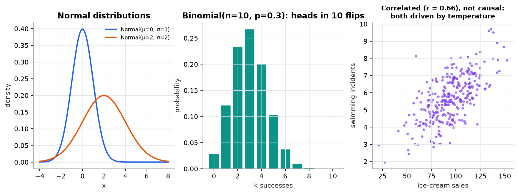
Right panel is synthetic: both variables are generated from temperature and do not affect each other, yet their correlation is 0.66.
3. The math
Symbols
| Symbol | Meaning |
|---|---|
| probability of event , between 0 and 1 | |
| probability that both and happen | |
| probability of given that happened | |
| expectation (mean) of random variable | |
| , | variance and standard deviation |
| mean of a distribution |
Core rules
The middle one is Bayes' rule: posterior = likelihood × prior / evidence.
Distributions you will meet
| Distribution | Describes | Mean | Variance |
|---|---|---|---|
| Bernoulli() | one yes/no outcome | ||
| Binomial(, ) | successes in trials | ||
| Categorical() | one of classes (or tokens) | ||
| Normal(, ) | sums of many small effects, measurement noise |
Worked example 1: Bayes' rule and the base rate
A disease affects 1% of people. A test detects it 95% of the time (sensitivity) and gives a false positive 5% of the time. You test positive. What is the chance you have the disease?
Only 16.1%. Out of 10,000 people, 95 sick people test positive and 495 healthy people test positive. The false positives swamp the true ones because healthy people are 99 times more common. This is exactly why accuracy misleads on imbalanced classification.
Worked example 2: expectation and variance
A die roll : . , so and .
Worked example 3: sampling error
A classifier gets 870 of 1,000 test examples right: accuracy . The standard error of a proportion is . A rough 95% interval is . A competing model scoring 0.88 on the same set is not clearly better.
4. Implementation
You will build the statistics that ML evaluation leans on, using only the Python standard library: variance, correlation, Bayes' rule, a bootstrap confidence interval, and a permutation test for "is model A really better than model B?". Each one reproduces a worked example above.
Build it from scratch
Mean and variance first. The sample=True branch divides by n − 1 (Bessel's correction): a sample's points sit closer to their own mean than to the true mean, so dividing by n underestimates the spread.
def mean(xs):
    return sum(xs) / len(xs)

def variance(xs, sample=True):
    m = mean(xs)
    ss = sum((x - m) ** 2 for x in xs)
    return ss / (len(xs) - 1 if sample else len(xs))   # n - 1: Bessel's correction
Predict: for [2, 4, 4, 4, 5, 5, 7, 9] (mean 5, squared deviations summing to 32), what are the population and sample variances?
Pearson correlation is covariance divided by both spreads, so it lands in [−1, 1] whatever the units.
def pearson(x, y):
    mx, my = mean(x), mean(y)
    cov = sum((a - mx) * (b - my) for a, b in zip(x, y))
    return cov / (sum((a - mx) ** 2 for a in x) * sum((b - my) ** 2 for b in y)) ** 0.5
Bayes' rule is worked example 1 as a function. The denominator is the total probability of a positive test, from both sick and healthy people.
def bayes(prior, sensitivity, false_positive_rate):
    evidence = sensitivity * prior + false_positive_rate * (1 - prior)   # P(positive)
    return sensitivity * prior / evidence
Predict: raise the prior from 1% to 10% and keep the test the same. Does P(disease | positive) roughly double, or more?
The bootstrap estimates uncertainty without a formula: resample the data with replacement many times, recompute the statistic each time, and read off the middle 95% of the results.
def bootstrap_ci(xs, stat=mean, n_boot=2000, alpha=0.05, rng=random):
    boots = sorted(stat(rng.choices(xs, k=len(xs))) for _ in range(n_boot))
    return boots[int(n_boot * alpha / 2)], boots[int(n_boot * (1 - alpha / 2)) - 1]
A permutation test asks: if the labels "A" and "B" meant nothing, how often would shuffling them produce a gap at least this large? That fraction is the p-value. The +1 on top and bottom keeps it from ever being exactly 0.
def permutation_test(a, b, n_perm=5000, rng=random):
    """Two-sided p-value for 'mean(a) - mean(b) is zero': shuffle the labels and count."""
    observed = abs(mean(a) - mean(b))
    pooled = a + b
    hits = 0
    for _ in range(n_perm):
        rng.shuffle(pooled)
        if abs(mean(pooled[:len(a)]) - mean(pooled[len(a):])) >= observed:
            hits += 1
    return (hits + 1) / (n_perm + 1)
Predict: you run the bootstrap on 870 correct out of 1,000. Should the interval match worked example 3's [0.849, 0.891]? Would it get narrower with 10,000 resamples, or with 10,000 test examples?
Answers
Population variance 32/8 = 4.0; sample variance 32/7 = 4.571. With a 10% prior: 0.95 × 0.1 / (0.095 + 0.045) = 0.679, about four times 0.161, not double, because false positives from the healthy group shrink in relative terms. The bootstrap gives about [0.850, 0.890], matching the formula. More resamples only make the estimate of the interval less noisy; more test examples make the interval itself narrower (by √n).
Use the library
The standard library already has these: statistics.mean, statistics.variance (sample, n − 1), statistics.pvariance (population), and statistics.correlation. For tests and intervals, SciPy is the usual tool:
from scipy import stats

stats.ttest_ind(a, b, equal_var=False)                      # Welch's t-test
stats.permutation_test((a, b), lambda x, y: x.mean() - y.mean(), n_resamples=5000)
stats.bootstrap((correct,), np.mean, confidence_level=0.95)
In NumPy, watch the default: np.var and np.std divide by n (ddof=0), while pandas .var() and .std() divide by n − 1. The scratch code made that choice explicit; libraries make it silently. (SciPy is not in this repo's dependencies; the script uses only the standard library.)
Run it
From guide/:
uv run code/00-foundations/stats_scratch.pymean 5.0, population var 4.0, sample var 4.5714
P(disease | positive) = 0.1610
CLT: std of 5000 sample means 0.3096, predicted σ/√30 = 0.3118
accuracy 0.870, bootstrap 95% CI [0.850, 0.890]
mean A 0.810, mean B 0.753, permutation p = 0.0040
r(ice cream, incidents) = 0.552 (confounder: temperature)
all checks match the statistics moduleThe CLT line checks worked example 2: a die has σ = 1.708, so the mean of 30 rolls should have spread 1.708/√30 = 0.312. All data is synthetic and seeded. Full script: code/00-foundations/stats_scratch.py. Figures: code/00-foundations/foundations.py.
5. Engineering
Every metric is an estimate. Report confidence intervals (bootstrap is simple and general), especially for small test sets or rare classes. Compare models on the same examples (paired comparisons are far more sensitive).
Base rates drive precision. When positives are rare, even a good classifier's alarms are mostly false. Choose thresholds and metrics with the base rate in mind.
Correlation versus causation. A predictive model exploits correlations; it doesn't learn what would happen if you intervened. Don't read coefficients or feature importances as causal effects. Estimating causal effects needs experiments (A/B tests) or causal-inference methods.
Sampling and representativeness. A model learns the distribution it was trained on. If production users differ (new regions, seasons, products), performance changes. That is distribution shift.
Watch outFailure modes. Ignoring base rates; treating a 0.5-point metric difference on 500 examples as real; drawing causal conclusions from observational data; training on a sample that doesn't represent production.
Common mistakes
- Confusing with (the prosecutor's fallacy).
- Assuming independence when events are linked.
- Reporting a single number without a sense of its uncertainty.
6. Knowledge check
Quiz: Probability and statistics
2% of transactions are fraud. A detector flags 90% of fraud and 10% of legitimate transactions. What is ? (3 decimals)
Practice exercise. 30% of emails are spam. "Winner" appears in 40% of spam and 2% of non-spam. What is ?
Solution
.
Implementation challenge. Simulate the disease example for base rates of 0.1%, 1%, 10%, and 50%, and plot . Explain the curve.
Summary
- Conditional probability updates beliefs with evidence; Bayes' rule flips the conditional and depends on the prior.
- Rare positives make even accurate tests produce mostly false alarms.
- Expectation is the long-run mean; variance is spread. Know Bernoulli, binomial, categorical, and normal.
- Every evaluation metric is an estimate with uncertainty.
- Correlation is not causation; predictive models capture correlations.
Next: The Python toolkit
Related: Naive Bayes · Classification metrics
Go deeper, code-first (AI Engineering from Scratch): Sampling Methods · Stochastic Processes
Parts of this lesson are adapted from AI Engineering from Scratch by Rohit Ghumare (MIT license, notice): Probability and Distributions, Statistics for Machine Learning.
Interview angle
A fraud model has 99% recall and a 1% false-positive rate. 0.1% of transactions are fraud. What fraction of flagged transactions are actually fraud?
Use Bayes' rule, or just count. Per million transactions: 1,000 are fraud, and 990 of them are flagged; 999,000 are legitimate, and 1% of those, 9,990, are flagged. Precision . Only about 9% of flags are real fraud, even though both component rates sound excellent. The false-positive rate applies to a population 999 times larger, so it dominates. What to say next: precision depends on prevalence, so the same model has different precision in markets with different fraud rates, and a validation set rebalanced to 50/50 would report a wildly optimistic precision. To improve it, lower the false-positive rate (higher threshold, better features) or route flags through a cheap review step, and always report precision at the production base rate.
Why do we minimize the negative log-likelihood instead of maximizing the likelihood directly?
They have the same optimum, because the logarithm is monotonic, but the log version is far easier to work with. The likelihood of i.i.d. data is a product, : with a million examples each around 0.5, that is , which underflows to exactly 0 in floating point. The log turns the product into a sum, , which is numerically stable and decomposes per example, so minibatch SGD works. Negating it gives a loss to minimize. It also has an information-theoretic meaning: the average negative log-likelihood is the cross-entropy between the data and the model, in nats. Common losses are special cases: squared error is the negative log-likelihood under Gaussian noise, binary cross-entropy under a Bernoulli model, and categorical cross-entropy under a categorical model.
Model B beats model A by 0.8 accuracy points on the same 1,000-example test set. Do you ship B?
Not on that evidence alone. At accuracy near 0.87 with , the standard error is , so a 95% interval is roughly ±2.1 points, and a 0.8-point gap sits well inside the noise. Because both models are scored on the same examples, use a paired analysis: look only at examples where they disagree and run McNemar's test, or bootstrap the accuracy difference by resampling test examples. Paired comparisons are much tighter than two independent intervals. Also ask: was this test set used during tuning (then it is optimistic for whichever model was tuned more), does B win on the slices that matter, and do latency, cost, and calibration favor it? If the gap matters commercially, collect more test data or run an online A/B test.
Users who adopt feature X churn 30% less. The PM wants to push every user into X. What do you say?
That is a correlation in observational data, and it can't tell us what pushing users into X would do. The likely confounder is engagement: highly engaged users both discover X and stay, the same way temperature drives both ice-cream sales and swimming incidents. There may also be selection (people who need X differ from those who don't) and reverse causation (users already planning to leave stop exploring features). To estimate the causal effect, run a randomized experiment: prompt a random half of eligible users toward X and compare churn between the two arms, not between adopters and non-adopters. If an experiment is impossible, causal-inference methods such as matching on pre-treatment engagement or difference-in-differences around a launch can help, but they rest on assumptions you must state. Expect the true effect to be much smaller than 30%.