Module 17: LLM evaluation 45 min9 min quick readLLMs
Evaluating LLM systems
Build an evaluation set, measure retrieval with recall@k, MRR, and nDCG, score answers for correctness and groundedness, use LLM judges carefully, track latency and cost, and compare system versions soundly.
Before this: The RAG pipeline, Classification metrics and thresholds, Probability and statistics
Quick read: the intuition, interactive visualization, summary, and interview questions. The math, implementation, engineering, and knowledge-check sections are hidden.
Mental model. An LLM system is a pipeline, so evaluate it like one: check each layer (retrieval, grounding, task quality, safety, operations) on a fixed set of realistic cases, and compare versions on the same cases. A demo that looks good is a sample size of one.
You will learn to
- Design an evaluation set with expected outputs, contexts, and failure categories.
- Compute recall@k, precision@k, MRR, and nDCG by hand.
- Score answers with exact match, token F1, rubrics, and groundedness checks.
- Use LLM-as-judge with its known biases in mind.
- Compare two system versions with paired statistics, alongside latency and cost.
Why it matters. Without evaluation, every prompt change is a guess and every model upgrade is a gamble. Evaluation turns "it seems better" into "it fixed 6 cases, broke 2, costs 47% more, and the difference is not yet statistically clear."
1. Intuition
Start with test cases: real or realistic user questions, each with what a good answer must contain, the documents that should be retrieved, and tags (topic, difficulty, adversarial). Fifty well-chosen cases beat five thousand random ones at first; grow the set from production failures.
Then measure by layer:
| Layer | Question | Example metrics |
|---|---|---|
| Retrieval | Did we fetch the right evidence? | recall@k, MRR, nDCG, context relevance |
| Grounding | Is every claim supported by the context? | claim support rate, citation correctness, faithfulness |
| Task quality | Is the answer right and useful? | exact match, F1, rubric score, human rating |
| Safety | Does it resist misuse? | harmful-content rate, prompt-injection success rate, privacy leaks |
| Operations | Can we afford and serve it? | p50/p95 latency, tokens/sec, error rate, cost per request, cache hit rate |
Failure categorization turns a score into a to-do list: retrieval misses mean fix search; unsupported claims mean fix grounding instructions or add verification; wrong formats mean fix schemas.
2. Visualization
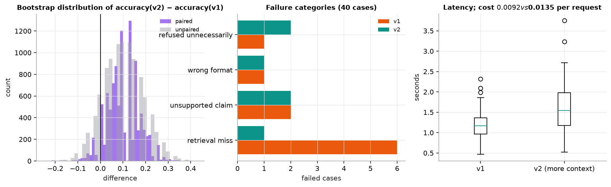
Synthetic evaluation of two versions on 40 cases. v2 sends more retrieved context: accuracy 0.75 → 0.85, but p95 latency rises from 1.99 s to 2.74 s and cost per request from about 0.9 to 1.35 cents (illustrative prices).
3. The math
Symbols
| Symbol | Meaning |
|---|---|
| whether the result at rank is relevant (graded relevance also works) | |
| total number of relevant items for the query | |
| rank of the first relevant result for query | |
| number of queries |
Retrieval metrics
IDCG is the DCG of the ideal ordering. nDCG rewards putting relevant results near the top.
Answer metrics
- Exact match: 1 if the normalized answer equals the reference.
- Token F1: precision and recall of answer tokens against reference tokens, then F1.
- Groundedness: fraction of the answer's claims supported by the provided context.
Worked example 1: ranking metrics
Five results with relevance ; two relevant documents exist ().
- recall@1 ; recall@3 ; recall@5 . precision@3 .
- Reciprocal rank: first relevant at rank 2, so .
- DCG@5 .
- IDCG@5 (relevant at ranks 1 and 2) .
- nDCG@5 .
Over four queries whose first relevant results are at ranks 1, 2, none, and 3: MRR .
Worked example 2: token F1
Reference "30 days from purchase" (4 tokens); answer "within 30 days" (3 tokens). Overlap: "30", "days" (2 tokens). Precision , recall , F1 . Exact match is 0 even though the answer is correct, which is why exact match alone undercounts.
Worked example 3: comparing versions properly
On the same 40 cases, v2 fixed 6 cases and broke 2, so accuracy rose from 0.75 to 0.85 (+0.10). A paired bootstrap (resampling cases and recomputing both versions on each resample) gives a 95% interval of . An unpaired bootstrap that ignores the pairing gives the wider . Both include 0: with 40 cases, a 10-point gain is promising but not conclusive. Add cases (especially in the categories that changed) before declaring victory, and weigh the 47% cost increase.
4. Implementation
The full script is code/17-llm-evaluation/eval_scratch.py (NumPy and stdlib only). It implements every metric this lesson uses, reproduces worked examples 1 to 3, and adds three that come up constantly in practice: claim-level faithfulness, pass@k for code, and calibration error. All cases are synthetic.
Build it from scratch
Step 1: ranking metrics. rels is the relevance of each returned result in rank order. Recall needs , the number of relevant items that exist, which the ranked list alone cannot tell you. Rank (1-based) is discounted by because Python counts from 0.
def recall_at_k(rels, k, R):
    return sum(rels[:k]) / R

def reciprocal_rank(rels):
    return next((1 / (i + 1) for i, r in enumerate(rels) if r), 0.0)   # 0 if nothing relevant

def ndcg_at_k(rels, k):
    dcg = sum(r / math.log2(i + 2) for i, r in enumerate(rels[:k]))   # rank i+1 -> log2(i+2)
    idcg = sum(r / math.log2(i + 2) for i, r in enumerate(sorted(rels, reverse=True)[:k]))
    return dcg / idcg if idcg else 0.0
Predict: a query returns [1, 1, 0, 0, 0] and there are 4 relevant documents in total. nDCG@5 computed this way is 1.0. Is the retriever perfect?
Step 2: exact match and token F1. Normalize first (lowercase, strip punctuation and articles) so formatting noise doesn't count as wrong. F1 counts shared tokens with multiplicity, which the Counter intersection does in one line.
def normalize(s):
    s = s.lower().translate(str.maketrans("", "", string.punctuation))
    return [t for t in s.split() if t not in {"a", "an", "the"}]

def token_f1(pred, ref):
    p, r = normalize(pred), normalize(ref)
    overlap = sum((Counter(p) & Counter(r)).values())   # shared tokens, counted with multiplicity
    if overlap == 0:
        return 0.0
    prec, rec = overlap / len(p), overlap / len(r)
    return 2 * prec * rec / (prec + rec)
Predict: the answer "not within 30 days" against the reference "within 30 days". F1 is high. Is the answer right?
Step 3: faithfulness. Split the answer into claims and ask, for each one, whether the retrieved context supports it. The score is the supported fraction. Frameworks such as RAGAS do this with an LLM or an NLI (entailment) model as the supported function; here a word-overlap rule stands in so the script runs offline.
def faithfulness(answer, context, supported):
    """`supported(claim, context) -> bool` is an NLI model or LLM judge in production."""
    claims = [c.strip() for c in re.split(r"(?<=[.!?])\s+", answer) if c.strip()]
    verdicts = [supported(c, context) for c in claims]
    return sum(verdicts) / len(claims), list(zip(claims, verdicts))
Predict: the overlap rule passes "Refunds never go to the original payment method." Why, and what kind of judge would catch it?
Step 4: pass@k for code. Generate samples per problem, run the tests, count passes. pass@k estimates the chance that at least one of samples passes: one minus the chance that all come from the failures. It is unbiased, unlike "pass rate of the first samples".
def pass_at_k(n, c, k):
    """Unbiased estimate: chance at least one of k samples passes, from n samples with c passing."""
    if n - c < k:
        return 1.0
    return 1 - math.comb(n - c, k) / math.comb(n, k)
For , , : , , so pass@5 .
Predict: what is pass@1 for , , without the formula?
Step 5: calibration. If the system reports confidence (to route low-confidence answers to a human, say), check it. Bin answers by stated confidence; in each bin compare average confidence with actual accuracy; weight the gaps by bin size.
def ece(conf, correct, bins=5):
    conf, correct = np.asarray(conf), np.asarray(correct)
    edges = np.linspace(0, 1, bins + 1)
    total = 0.0
    for lo, hi in zip(edges[:-1], edges[1:]):
        m = (conf > lo) & (conf <= hi)
        if m.any():                               # weight each bin's |accuracy - confidence| by its size
            total += m.mean() * abs(correct[m].mean() - conf[m].mean())
    return total
On the script's ten synthetic answers: bin (0.4, 0.6] holds 2 answers, confidence 0.575, accuracy 0.5, gap 0.075. Bin (0.6, 0.8] holds 4, confidence 0.725, accuracy 0.25, gap 0.475. Bin (0.8, 1.0] holds 4, confidence 0.9, accuracy 0.75, gap 0.15. ECE .
Predict: a system always says 50% confidence and is right half the time. What is its ECE, and is it useful?
Step 6: paired bootstrap. Resample cases with replacement, and use the same resampled cases for both versions. That keeps each case's difficulty attached to both scores, which is what makes the interval narrow enough to be useful.
def paired_bootstrap(a, b, n_boot=10_000, seed=0):
    rng = np.random.default_rng(seed)
    a, b = np.asarray(a), np.asarray(b)
    idx = rng.integers(0, len(a), (n_boot, len(a)))   # resample CASES; both versions share them
    return np.percentile(b[idx].mean(1) - a[idx].mean(1), [2.5, 97.5])
Predict: resample a and b with separate indices. Does the interval get wider or narrower?
Use the library
The metric math is small; the libraries add datasets, judges, and reporting:
from sklearn.metrics import ndcg_score                    # graded relevance, batched queries
ndcg_score([[0, 1, 0, 1, 0]], [[5, 4, 3, 2, 1]])          # true relevance, system scores -> 0.651

import evaluate                                           # pip install evaluate
squad = evaluate.load("squad")                            # exact match and token F1, normalized like step 2
RAGAS implements step 3 (faithfulness) plus context precision and recall with an LLM judge; DeepEval wraps metrics as pytest-style tests for CI; Inspect and promptfoo run eval suites against models and prompts. Whatever you use, freeze the judge model and its prompt, log every judge rationale, and check the judge against at least a hundred human labels before trusting its numbers.
Run it
uv run code/17-llm-evaluation/eval_scratch.pyKey lines of output:
recall@1,3,5: [0.0, 0.5, 1.0] RR 0.500  nDCG@5 0.651
MRR over 4 queries (first relevant at 1, 2, none, 3): 0.458
EM 0  F1 0.571  |  EM('The 30 days of purchase.') 1
  UNSUPPORTED | A store credit option is also available.
faithfulness = 0.67
pass@1 = 0.150  pass@5 = 0.601  pass@10 = 0.895
mean confidence 0.76, accuracy 0.50, ECE 0.265
accuracy 0.75 -> 0.85; paired 95% CI for the gain [-0.025, +0.225]
The first three lines are worked examples 1 and 2. The last line rebuilds worked example 3's shape (6 fixed, 2 broken out of 40) and gets the same interval, which includes 0. The figure, failure categories, latency, and cost comparison are in code/17-llm-evaluation/eval.py.
5. Engineering
LLM-as-judge. Useful for scaling rubric grading, but judges have known biases: position bias (preferring the first answer shown), verbosity bias (preferring longer answers), self-preference (favoring their own model family), and inconsistency across runs. Mitigate with clear rubrics, randomized order, reference answers, pairwise comparisons, and regular agreement checks against human labels.
Eval-driven development. Write the eval cases before the change, the way you would write a failing test: a new prompt, model, or agent step ships only when it fixes the target cases without regressing the rest. Keep the suite in version control next to the code, run a fast subset in CI on every change and the full suite before release, and turn every production incident into a new case.
Human evaluation remains the ground truth for usefulness and tone; sample regularly and measure agreement between raters.
Offline versus online. Offline evals gate releases. Online signals (thumbs up or down, user corrections, task completion, escalation rate) and A/B tests measure real impact. Feed production failures back into the offline set.
Operational metrics matter as much as quality: report p50 and p95 latency, tokens per second, error and timeout rates, cost per request, and cache hit rate for every version.
Safety evaluation: include adversarial cases such as prompt injection in retrieved documents, attempts to extract system prompts or other users' data, and requests for disallowed actions.
Watch outFailure modes. Evaluating only fluency; tiny or unrepresentative test sets; overfitting prompts to the eval set; LLM judges grading their own outputs; ignoring cost and latency; comparing versions on different cases.
Common mistakes
- Reporting a single aggregate score without failure categories.
- Treating a 2-point change on 50 cases as meaningful.
- Using only exact match for free-form answers.
- Letting the eval set go stale as the product changes.
- Letting judge or parsing failures become missing values that silently drop out of the average. Count them as failures and report them.
6. Knowledge check
Quiz: Evaluating LLM systems
Relevance of the top 4 results is and there are 4 relevant documents in total. What is recall@4?
Practice exercise. Results have relevance with . Compute recall@3, precision@3, reciprocal rank, and nDCG@5.
Solution
recall@3 ; precision@3 ; reciprocal rank . DCG@5 . With the ideal ordering puts three relevant items first, but only two were retrieved; using the retrieved list's ideal ordering gives IDCG and nDCG . (If IDCG is computed from all 3 relevant documents, IDCG and nDCG . State which convention you use.)
Implementation challenge. Build a 30-case evaluation set for the RAG script's documents. For each case store the question, the expected answer, and the expected source. Score retrieval recall@3, answer token F1 against your expected answers (using any LLM or a template answer), and tag every failure with a category.
Summary
- Evaluate each layer: retrieval, grounding, task quality, safety, and operations.
- recall@k and precision@k count hits; MRR rewards the first hit; nDCG rewards good ordering.
- Use token F1 and rubrics for free-form answers; check claims against context for groundedness.
- LLM judges scale grading but are biased; calibrate them against humans.
- Compare versions on the same cases with paired statistics, and always report latency and cost.
Next: LLM inference
Related: The RAG pipeline · Classification metrics · Securing AI systems
Go deeper, code-first (AI Engineering from Scratch): Natural Language Inference — Textual Entailment · Long-Context Evaluation — NIAH, RULER, LongBench, MRCR · Evaluation: Benchmarks, Evals, LM Harness · Benchmarks: SWE-bench, GAIA, AgentBench · METR Time Horizons and External Capability Evaluation · Language Model Evaluation Harness · Classical Metrics · Leaderboard Aggregation
Parts of this lesson are adapted from AI Engineering from Scratch by Rohit Ghumare (MIT license, notice): RAG Evaluation: Precision, Recall, MRR, nDCG, Faithfulness, Answer Relevance, Code Exec Metric, Perplexity and Calibration, LLM Evaluation — RAGAS, DeepEval, G-Eval, Evaluation & Testing LLM Applications, Eval-Driven Agent Development.
Interview angle
How would you evaluate an LLM feature before launch?
Build a fixed evaluation set and measure each layer of the system on it, then gate the release on those numbers. Start with 50 to 200 realistic cases from real or expected user queries, tagged by topic, difficulty, and adversarial type, each with an expected answer or rubric and, for RAG, the expected source documents. Measure retrieval (recall@k, MRR), grounding (are claims supported by the retrieved context?), task quality (exact match, token F1, or rubric scores from humans or a calibrated LLM judge), safety (prompt-injection and harmful-content cases), and operations (p50 and p95 latency, cost per request). Categorize every failure so scores become a to-do list. Compare candidate versions on the same cases with paired statistics. Before full launch, run a shadow test or a small A/B test with online signals such as thumbs, escalations, and task completion, and feed production failures back into the offline set.
Explain recall@k, MRR, and nDCG. When would you use each for a RAG retriever?
Recall@k asks "did the relevant items make it into the top ?" MRR asks "how high was the first relevant item?" nDCG asks "how good was the whole ordering?" Take relevance with two relevant documents. Recall@3 and recall@5 . The reciprocal rank is because the first hit is at rank 2. DCG@5 ; the ideal ordering gives , so nDCG@5 . For RAG, recall@k at the you actually put in the prompt is the primary metric, because the generator sees all chunks: if the evidence isn't there, nothing downstream can fix it. MRR suits single-answer lookups and tight . nDCG matters with graded relevance, or when the model seems to weight earlier chunks more.
Your LLM judge says version 2 is clearly better, but users are complaining more. What is going on?
The judge is probably measuring something other than what users value. LLM judges have known biases: verbosity (preferring longer answers), position (preferring whichever answer is shown first in pairwise comparisons), self-preference (favoring outputs from their own model family), and run-to-run inconsistency. If v2 gives longer, more confident answers, a judge can reward it while users find it slower and less precise. Diagnose by sampling 50 to 100 cases, having humans grade them blind, and measuring judge-human agreement. Then look at where they disagree. Fix the judge: a specific rubric with a reference answer, pairwise comparisons with randomized order (or both orders), a length-controlled analysis, and a judge from a different model family. Also check the evaluation set for staleness, since user questions may have drifted from the offline cases, and compare latency and cost, which users feel and the judge ignores.
Version 2 fixed 6 cases and broke 2 on a 40-case evaluation set. Do you ship it?
Not on accuracy evidence alone; the improvement isn't statistically clear yet. Accuracy went from 0.75 to 0.85, a gain of 0.10. Only the 8 cases that changed carry information about the difference. A paired bootstrap, resampling cases and recomputing both versions on each resample, gives a 95% interval of about , which includes zero. An exact sign test on the 6-versus-2 split gives a two-sided p-value of . Ignoring the pairing makes the interval wider, so always pair. Then weigh the other dimensions: here v2 also raised p95 latency and cost per request. My answer: grow the evaluation set (several hundred cases makes a 10-point gain much easier to resolve), read the 2 regressions to see if they're severe, and if shipping, ramp gradually with online metrics.