Module 4: Classification 35 min7 min quick readClassical ML
Logistic regression
Turn a linear score into a probability with the sigmoid, train it with cross-entropy, and extend it to many classes with softmax.
Before this: Linear regression, Probability and statistics
Quick read: the intuition, interactive visualization, summary, and interview questions. The math, implementation, engineering, and knowledge-check sections are hidden.
Mental model. Compute a linear score, exactly like linear regression, then squeeze it into a probability between 0 and 1 with the sigmoid function. Train by making the probability of the correct label as high as possible.
You will learn to
- Compute a logit, a sigmoid probability, and binary cross-entropy by hand.
- Interpret weights as changes in log-odds.
- Derive the gradient and take a training step.
- Extend to classes with softmax and categorical cross-entropy.
- Explain why the decision boundary is linear and when that is a problem.
Why it matters. Logistic regression is the default baseline for classification: fast, interpretable, and usually well calibrated. Its pieces (logits, sigmoid, softmax, cross-entropy) are exactly the output layer of every neural classifier and every language model.
1. Intuition
Linear regression outputs any real number, but a probability must lie in . Logistic regression keeps the linear score, called the logit , and passes it through the sigmoid :
- very negative gives a probability near 0,
- gives exactly 0.5,
- very positive gives a probability near 1.
The boundary where the model is undecided () is where , a straight line (or flat plane) in feature space.
Training uses cross-entropy: the negative log of the probability the model gave the correct label. Predicting 0.9 for a true positive costs ; predicting 0.01 costs . Confident mistakes are punished hard.
2. Visualization
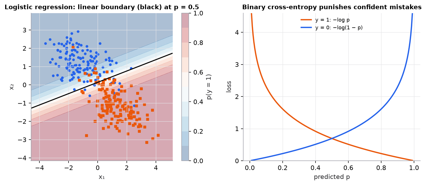
Synthetic data. Probability changes smoothly across the boundary; the model is most uncertain near the black line.
3. The math
Symbols
| Symbol | Meaning | Shape |
|---|---|---|
| features | ||
| weights and bias (parameters) | , scalar | |
| logit (log-odds), | scalar | |
| predicted probability of class 1, | scalar | |
| true label | scalar | |
| , | logit and probability for class (multiclass) |
Model and loss
Log-odds interpretation
Rearranging the sigmoid: . Increasing feature by one unit adds to the log-odds, which multiplies the odds by .
Gradient
Using and the chain rule, the sigmoid's derivative cancels:
Same form as linear regression: (prediction − target) × input.
Multiclass: softmax and categorical cross-entropy
Worked example 1: one prediction
One feature (hours studied) with , . A student studied hours.
- Logit: .
- Probability: .
- If they passed (): . If they failed (): .
- Gradient for : , so a gradient step increases .
- Odds: . Each extra hour multiplies the odds by .
Worked example 2: softmax
Logits . Exponentials , sum . Probabilities . If class 0 is correct, .
4. Implementation
You will build binary logistic regression and its multi-class form (softmax regression) from scratch in NumPy, with the two numerical guards every real implementation has, then confirm the probabilities match scikit-learn.
Build it from scratch
The sigmoid from section 3, written so it never overflows. np.exp(1000) is infinity, so the naive 1 / (1 + np.exp(-z)) warns for large negative z. Computing exp(-|z|) keeps the exponent at or below zero for every input.
def sigmoid(z):
    # Stable for large |z|: never calls exp on a large positive number
    e = np.exp(-np.abs(z))                                 # always in (0, 1]
    return np.where(z >= 0, 1 / (1 + e), e / (1 + e))

def bce(y, p, eps=1e-12):
    p = np.clip(p, eps, 1 - eps)                           # log(0) guard
    return -np.mean(y * np.log(p) + (1 - y) * np.log(1 - p))
Predict: without the clip, what is the loss on one example where the model outputs p = 1.0 exactly but the label is 0?
Training is gradient descent on mean binary cross-entropy. The gradient is the tidy from worked example 1, averaged over rows: the same shape as linear regression's, with a probability in place of a raw prediction.
def fit_logistic(X, y, lr=0.5, steps=3000):
    n, d = X.shape
    w, b = np.zeros(d), 0.0
    for _ in range(steps):
        p = sigmoid(X @ w + b)                              # [n] probabilities
        w -= lr * X.T @ (p - y) / n                         # gradient of mean BCE: (p - y) x
        b -= lr * np.mean(p - y)
    return w, b
Predict: if the training data is perfectly separable (some line puts every 0 on one side and every 1 on the other), what happens to w as you keep training?
Softmax turns k logits into k probabilities. Subtracting each row's maximum first changes nothing mathematically (it cancels in the ratio) but keeps exp from overflowing.
def softmax(Z):
    Z = Z - Z.max(axis=1, keepdims=True)                   # subtract row max: same result, no overflow
    E = np.exp(Z)
    return E / E.sum(axis=1, keepdims=True)
Softmax regression has one weight column per class, W of shape [d, k]. With one-hot labels Y, the gradient has exactly the binary form, (P − Y) times the inputs.
def fit_softmax(X, y, k, lr=0.5, steps=3000):
    n, d = X.shape
    W, b = np.zeros((d, k)), np.zeros(k)
    Y = np.eye(k)[y]                                        # one-hot, [n, k]
    for _ in range(steps):
        P = softmax(X @ W + b)                              # [n, k]
        W -= lr * X.T @ (P - Y) / n                         # same (p - y) x shape as the binary case
        b -= lr * (P - Y).mean(axis=0)
    return W, b
Predict: softmax([[1000, 1001, 1002]]) with and without the max subtraction. What does each return?
Answers
Without the clip, p = 1.0 with y = 0 gives −log(0) = infinity, and one bad example turns the whole mean loss into inf; with eps = 1e-12 it is a large but finite 27.6. On separable data, w grows without bound: making |z| larger always lowers the loss a little, so plain gradient descent never stops. That is one reason libraries add L2 regularization by default. Without the shift, exp(1000) overflows to inf and you get inf / inf = nan. With it, the logits become [−2, −1, 0] and the output is [0.090, 0.245, 0.665].
Use the library
from sklearn.linear_model import LogisticRegression
from sklearn.pipeline import make_pipeline
from sklearn.preprocessing import StandardScaler

clf = make_pipeline(StandardScaler(), LogisticRegression(C=1.0, max_iter=1000))   # C = 1/λ (L2)
clf.fit(X_train, y_train)
proba = clf.predict_proba(X_test)[:, 1]   # probabilities; choose the threshold separately
What the library adds: L2 regularization on by default (C is the inverse strength, so smaller C means stronger shrinkage, the fix for the separable case), a second-order solver (L-BFGS) that needs no learning rate, and automatic softmax when y has more than two classes. To compare with the scratch code, the script turns the penalty off with C=np.inf.
Run it
From guide/:
uv run code/04-classification/logistic_scratch.pysigmoid(-1000), sigmoid(0), sigmoid(1000) = [0. 0.5 1. ]
binary: BCE 0.4567, accuracy 0.824, w = [ 2.636 -0.871 0.114 1.285]
sklearn (no penalty): w = [ 2.636 -0.871 0.114 1.285]
softmax: rows sum to 1: True, accuracy 0.963
sklearn multinomial accuracy 0.958
checks pass: scratch probabilities match scikit-learnBoth datasets are synthetic (make_classification, make_blobs). The worked examples, the decision-boundary figure, and the cross-entropy figure come from code/04-classification/classification.py. Full scratch script: code/04-classification/logistic_scratch.py.
5. Engineering
Good use cases. Baselines for any classification problem; sparse high-dimensional data such as TF-IDF text; credit and risk models that must be explained; any setting where calibrated probabilities matter.
Regularization. scikit-learn applies L2 by default with strength C = 1/λ (smaller C means more regularization). Without regularization, perfectly separable data drives weights to infinity.
Preprocessing. Scale features (for the optimizer and the penalty); one-hot categoricals; add interaction or polynomial features if the boundary should curve.
Cost. Training is fast (convex, solved with L-BFGS or similar); inference is one dot product.
Thresholds are separate. predict uses 0.5, which is rarely the right business threshold. Use predict_proba and choose the threshold from error costs (next lesson).
Watch outFailure modes. Nonlinear boundaries (XOR-like patterns) that a linear score can't separate; perfect separation without regularization; correlated features making weights unstable and hard to interpret; class imbalance making the 0.5 threshold useless.
Common mistakes
- Using MSE instead of cross-entropy (the loss becomes non-convex in and gradients vanish).
- Computing
log(sigmoid(z))directly for large negative ; use stable library losses. - Reading coefficients without scaling features first.
- Treating predicted probabilities as calibrated without checking.
6. Knowledge check
Quiz: Logistic regression
A logistic model has logit . What probability does it predict?
Practice exercise. With , , and , compute , , and the loss if .
Solution
. . Loss for : .
Implementation challenge. Train fit_logistic on a synthetic 2D dataset, check your weights against scikit-learn with penalty=None, and plot the decision boundary .
Summary
- Logit ; probability ; the boundary is linear.
- Binary cross-entropy is of the probability of the true label; confident mistakes cost a lot.
- The gradient is , the same shape as linear regression.
- Each weight changes the log-odds; is the odds multiplier.
- Softmax plus categorical cross-entropy generalizes to many classes and is the output layer of neural classifiers and LLMs.
Next: Classification metrics and thresholds
Related: Linear regression · Forward pass · Model card: logistic regression
Parts of this lesson are adapted from AI Engineering from Scratch by Rohit Ghumare (MIT license, notice): Logistic Regression.
Interview angle
Why use cross-entropy rather than MSE to train logistic regression?
Two reasons. With a sigmoid output, MSE is non-convex in the weights, so optimization can stall on flat regions. More importantly, its gradient vanishes exactly when the model is confidently wrong: the MSE gradient with respect to the logit is , so if but , the factor kills the signal. Cross-entropy's gradient with respect to the logit is simply because the term cancels, so a confident mistake gets a gradient near , the strongest possible push. Cross-entropy is also the negative log-likelihood of a Bernoulli model, so minimizing it is maximum likelihood, it's convex for logistic regression, and it tends to produce calibrated probabilities. Squared error on probabilities (the Brier score) remains a fine evaluation metric.
Interpret a logistic regression coefficient of 0.7 on a standardized feature.
A one-standard-deviation increase in that feature, holding the others fixed, adds 0.7 to the log-odds, which multiplies the odds by : roughly doubles them. It does not mean the probability rises by 0.7 or by any fixed amount; the effect on probability depends on the starting point. From (odds 1), the odds become 2.01, so . From (odds 0.053), the odds become 0.106, so . Caveats an interviewer expects: "holding others fixed" is unrealistic when features are correlated, and correlation makes individual coefficients unstable; regularization shrinks coefficients toward zero, so they are biased estimates; and none of this is causal. Coefficients on unstandardized features aren't comparable in magnitude.
While training an unregularized logistic regression, the weights keep growing and the training loss approaches zero. What's happening?
The training data is linearly separable (or nearly so). If some classifies every example correctly, scaling it up by any factor still classifies them correctly and pushes every closer to 0 or 1, which always lowers cross-entropy. So the unregularized optimum is at infinity: weights grow without bound, predicted probabilities become 0 and 1, and coefficients and their standard errors are meaningless. It's common with many features relative to examples (sparse text), or with a leaky feature that perfectly predicts the label, which is worth checking first. Fix: add regularization (scikit-learn's default is L2 with C = 1, where smaller C means stronger), which gives a finite, unique solution, and tune C by cross-validation. Then check calibration, since overconfident probabilities are the symptom downstream users will notice.
Logits are [2, 1, 0.1] and the true class is 1. Compute the cross-entropy loss and its gradient with respect to the logits.
Softmax: , , , sum , so . Loss . The gradient of softmax cross-entropy with respect to the logits is : push the confidently wrong class 0 down hardest, push the true class up, and nudge class 2 down slightly. It's the same form as the binary case, . Implementation follow-up: compute the loss directly from logits with log-sum-exp, , subtracting first so large logits don't overflow. PyTorch's cross_entropy does exactly this when given raw logits, which is why you should not apply softmax yourself before calling it.