Module 15: Large language models 35 min10 min quick readLLMs
Scaling laws
Predict pretraining loss from parameters and tokens, find the compute-optimal model size for a FLOP budget, and explain why production models are deliberately over-trained.
Before this: Tokenization and pretraining, The transformer architecture
Quick read: the intuition, interactive visualization, summary, and interview questions. The math, implementation, engineering, and knowledge-check sections are hidden.
Mental model. Training a language model is like filling a bucket with two taps: one labelled parameters and one labelled data. Each tap gives diminishing returns, and your budget pays for the water from both. Scaling laws are the measured flow rates. They tell you how to split the budget so the bucket fills highest, and how much is left in the bucket that no tap can fill.
You will learn to
- Estimate training compute with .
- Evaluate the Chinchilla loss law for a given model.
- Derive the compute-optimal and for a budget and explain why the "20 tokens per parameter" rule is approximate.
- Explain why models meant for heavy inference are trained far past compute-optimal.
- Distinguish smooth loss scaling from apparently sudden "emergent" benchmark jumps.
Why it matters. Pretraining runs cost millions of dollars, so labs fit scaling laws on small runs and extrapolate before committing. The same reasoning answers everyday questions: why an 8B model trained on 15 trillion tokens beats an older 70B model at serving time, and why "just make it bigger" stopped being the whole story in 2022.
1. Intuition
Pretraining minimises next-token cross-entropy (see tokenization and pretraining). Plot that loss against model size, data size, or compute on log-log axes and you get remarkably straight lines: power laws (Kaplan et al., 2020).
Three ideas carry the lesson:
- Compute is the budget. A training step on one token costs about 2 FLOPs per parameter forward and 4 backward, so a run costs FLOPs for parameters and tokens. For a fixed , a bigger model means fewer tokens.
- Both knobs have diminishing returns, and there is a floor. A tiny model can't hold enough knowledge no matter how long you train it. A huge model trained on too little text hasn't seen enough to use its capacity. The loss never reaches zero, because text itself is unpredictable.
- There is a best split for each budget. Kaplan's 2020 fits suggested pushing model size hard, and GPT-3 (175B parameters, 300B tokens) followed that. Hoffmann et al. (2022) re-ran the experiment with learning-rate schedules matched to each run's length and found models should be much smaller and trained on much more data. Their 70B Chinchilla, trained on 1.4 trillion tokens with similar compute to the larger Gopher, outperformed it. The rule of thumb that came out: about 20 tokens per parameter.
Then the twist. Compute-optimal minimises training cost for a given loss. But a deployed model is run billions of times, and inference cost scales with . So it pays to train a smaller model on far more tokens than compute-optimal: you spend a bit more training compute for the same quality and save on every request afterwards (Sardana and Frankle, 2024). Llama 3 8B was trained on about 15 trillion tokens, roughly 1,900 tokens per parameter.
NoteScaling laws predict loss, a smooth continuous quantity. Benchmarks scored by exact match can look like they jump suddenly at some size ("emergence"). Schaeffer et al. (2023) showed many such jumps disappear under continuous metrics. Plan with loss; treat sudden capability claims with care.
2. Visualization
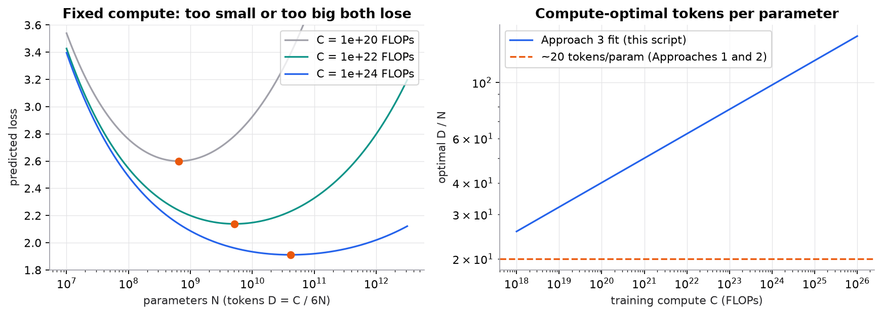
Left: along each fixed-compute line, a model that is too small is starved of capacity and one that is too big is starved of data. Right: with the published Approach 3 constants, the optimal ratio drifts with budget instead of sitting at 20.
Try it (in code/15-llms/scaling_laws.py; predict first, then run):
- Set
BETA = ALPHA = 0.34. Predict what happens to the right panel's line. (The exponent becomes 0.5, so and grow at the same rate and is constant.) - Double
E. Do the optimal and move? (No. The floor shifts every loss equally and doesn't change the argmin.) - In the over-training table, add
shrink = 100. How much loss do you give up for a model 100 times cheaper to serve? - Add Llama 3 70B (70e9 parameters, 15e12 tokens) to the first table and compare its predicted loss with Llama 3 8B's.
3. The math
Symbols
| Symbol | Meaning | Units |
|---|---|---|
| model parameters (non-embedding, in the original fits) | count | |
| training tokens | count | |
| training compute | FLOPs | |
| predicted pretraining loss | nats per token | |
| irreducible loss: the entropy of text itself | nats | |
| scale and exponent of the model-size term | fitted | |
| scale and exponent of the data term | fitted | |
| compute-optimal parameters and tokens for budget | count |
The law and the budget
Hoffmann et al.'s parametric fit (their Approach 3): , , , , .
The compute-optimal split
Substitute and set :
With and , the exponent is : grows as and as . Data should grow slightly faster than parameters, so rises with .
Key distinctionThe paper estimated the optimum three ways. Approaches 1 and 2 give and growing at about the same rate, with roughly 20 tokens per parameter around Chinchilla's budget. The Approach 3 constants above give a ratio that drifts from about 40 at FLOPs to about 150 at . Later replication work found issues in the original Approach 3 fit. Treat "20 tokens per parameter" as an order-of-magnitude rule, not a constant of nature.
Worked example: the optimum at C = 10^24 FLOPs
- .
- .
- .
- : ; ; .
- , about 41.3B parameters.
- , about 4.0T tokens, so .
- Loss: ; ; .
Worked example: Chinchilla and the cost of over-training
Chinchilla, , : FLOPs. , , so .
Now keep but shrink the model 10× from the optimum: B, T. The script prints , a loss increase of . In exchange, every generated token costs FLOPs: instead of , a 10× saving for the model's whole serving life. For a model served at scale, that trade usually wins.
4. Implementation
Build it from scratch
The full script is code/15-llms/scaling_laws.py (NumPy only). The law and the budget are two one-line functions. Writing them separately keeps "how good" and "how expensive" apart.
def loss(N, D):
    return E + A / N**ALPHA + B / D**BETA      # floor + model-size term + data term

def flops(N, D):
    return 6 * N * D                           # ~2ND forward + ~4ND backward
Predict: GPT-3 has 175B parameters and 300B tokens. Which term, model size or data, contributes more to its predicted loss? (Data: versus . That imbalance is the undertraining Chinchilla pointed out.)
The optimum comes from the closed form. A brute-force grid over checks the calculus, so a wrong exponent fails loudly.
def optimal_closed_form(C):
    G = (ALPHA * A / (BETA * B)) ** (1 / (ALPHA + BETA))
    N = G * (C / 6) ** (BETA / (ALPHA + BETA))
    return N, C / (6 * N)

def optimal_grid(C):
    Ns = np.logspace(6, 14, 20_001)            # brute force check of the calculus
    return Ns[np.argmin(loss(Ns, C / (6 * Ns)))]
Predict: if you multiply by 100, by what factor does grow? (. The table confirms it: 5.16B at , 41.3B at .)
Over-training holds fixed and moves along the same line: divide , multiply by the same factor.
for shrink in [1, 2, 4, 10]:
    N, D = N_opt / shrink, D_opt * shrink
    print(f"  N = N*/{shrink:<2}  N={N / 1e9:6.1f}B  D={D / 1e12:6.2f}T  loss={loss(N, D):.4f}  "
          f"(+{loss(N, D) - loss(N_opt, D_opt):.4f})  inference FLOPs/token {2 * N:.2e}")
Predict: is the loss penalty for shrinking 2× half the penalty for shrinking 4×? (No. Near the minimum the curve is flat, so the penalty grows roughly with the square of the log distance: 0.005, then 0.021.)
Use the library
Nobody needs a library to evaluate a power law. The real work is fitting one: train a grid of small models, record final losses, and fit by minimising a robust loss (Hoffmann et al. used a Huber loss on log-loss) with scipy.optimize.minimize:
from scipy.optimize import minimize

def fit(runs):                                   # runs: list of (N, D, final_loss) from your small models
    N, D, L = map(np.array, zip(*runs))
    def objective(p):
        a, b, e, alpha, beta = p                 # fit log A, log B, log E for stability
        pred = np.logaddexp.reduce([a - alpha * np.log(N), b - beta * np.log(D), np.full_like(N, e)])
        r = pred - np.log(L)
        return np.where(abs(r) < 1e-3, 0.5 * r**2, 1e-3 * (abs(r) - 0.5e-3)).sum()   # Huber
    return minimize(objective, x0=[6, 6, 0.5, 0.3, 0.3], method="L-BFGS-B").x
What the fit adds beyond our script: the constants are specific to a dataset, tokenizer, and architecture. Better data or a better optimizer shift them. Refit on your own setup before extrapolating; use multiple starting points, since the fit is sensitive.
Run it
From guide/:
uv run code/15-llms/scaling_laws.py=== predicted loss for three public (N, D) pairs ===
GPT-3 N= 175B D= 0.30T D/N= 2 C=3.15e+23 loss=2.002
Chinchilla N= 70B D= 1.40T D/N= 20 C=5.88e+23 loss=1.937
Llama 3 8B N= 8B D=15.00T D/N= 1875 C=7.20e+23 loss=1.949
=== compute-optimal split under the Approach 3 fit ===
C=1e+20 N*= 0.64B D*= 25.8B D/N= 40.1 loss=2.600
C=1e+22 N*= 5.16B D*= 323.0B D/N= 62.6 loss=2.139
C=1e+24 N*= 41.30B D*= 4035.8B D/N= 97.7 loss=1.911
...
N = N*/10 N= 4.1B D= 40.36T loss=1.9722 (+0.0610) inference FLOPs/token 8.26e+09These are predictions from a law fitted to one dataset, not measured losses of those models; different data and tokenizers make cross-model loss comparisons meaningless. The useful reading is relative: an 8B model trained on 15T tokens lands close to a 70B model trained on 1.4T, at a ninth of the inference cost.
5. Engineering
Using scaling laws in practice.
- Choosing a base model to serve: if traffic is high, prefer the smaller model trained on more tokens. Inference FLOPs per token are about .
- Planning a pretraining run: fit the law on runs at to of your budget, extrapolate, and check against one mid-size run before committing.
- Fine-tuning: scaling laws describe pretraining loss. Fine-tuning data needs are much smaller and governed by task difficulty, not by .
What shifts the curves. Data quality and deduplication, the tokenizer, optimizer and learning-rate schedule, and architecture changes all move the constants. Mixture-of-experts models decouple total from active parameters, so compute laws are written in active parameters. Labs increasingly hit a data limit: high-quality web text is finite, so repeated epochs, synthetic data, and multimodal data now matter.
Post-training and inference compute. Many capabilities that users notice (instruction following, reasoning with long chains of thought) come from post-training and from spending more compute at inference time, not only from pretraining scale. Pretraining laws don't predict those directly.
Watch outExtrapolating several orders of magnitude from a handful of small runs is fragile. A schedule that is mis-tuned at small scale (as in Kaplan's original fits) bends the whole curve.
Common mistakes
- Treating "20 tokens per parameter" as exact or as the best choice for a deployed model.
- Comparing predicted or reported losses across models with different tokenizers or data.
- Counting embedding parameters as in a small model, where they are a large fraction and distort the fit.
- Reading an exact-match benchmark jump as a phase change without checking a continuous metric.
- Forgetting that ignores attention FLOPs, which matter at long context.
6. Knowledge check
Quiz: Scaling laws
Using , how many FLOPs does it take to train a 7B-parameter model on 2 trillion tokens? Give the answer in units of FLOPs.
Practice exercise. You have FLOPs. Using "20 tokens per parameter", what and do you pick? How many tokens per parameter would Llama-3-style over-training at 1,000 tokens per parameter imply for the same budget, and what ?
Solution
With : , so and (22.4B). (447B tokens).
With : , so , (3.2B) and (3.2T tokens). A model about 7× cheaper to serve, at some loss cost.
Implementation challenge. Add a function that, given a target loss and a lifetime inference volume tokens, finds the that minimises total FLOPs subject to . Report the optimal tokens per parameter for and .
Solution
For each on a log grid, solve the data term for : , so (skip where the right side is : that model can never reach ). Compute total FLOPs and take the argmin.
def cheapest(L_target, T_inf):
    Ns = np.logspace(8, 12, 4001)
    gap = L_target - E - A / Ns**ALPHA
    ok = gap > 0
    D = (B / gap[ok]) ** (1 / BETA)
    total = 6 * Ns[ok] * D + 2 * Ns[ok] * T_inf
    i = np.argmin(total)
    return Ns[ok][i], D[i]
With you recover the compute-optimal point; as grows, the optimum moves to smaller and many more tokens per parameter, the Sardana and Frankle result.
Summary
- Training compute is about ; the Chinchilla law predicts loss from and .
- For a fixed budget the best split puts parameters and tokens on nearly equal growth; "20 tokens per parameter" is a rough headline, not a constant.
- Models served at scale are over-trained on purpose: a small loss cost buys large, lasting inference savings.
- Scaling laws predict smooth loss; many "emergent" jumps are artefacts of discontinuous metrics.
- Constants depend on data, tokenizer, and recipe; refit before you extrapolate.
Next: Open models: architecture walkthroughs
Related: Mixture of experts · Tokenization and pretraining · LLM inference
Parts of this lesson are adapted from AI Engineering from Scratch by Rohit Ghumare (MIT license, notice): Scaling Laws.
Interview angle
What did Chinchilla change about how we train LLMs?
Before 2022 the common reading of Kaplan's scaling laws was "grow the model, data matters less," so GPT-3 used 175B parameters on only 300B tokens, under 2 tokens per parameter. Hoffmann and colleagues trained hundreds of models with learning-rate schedules matched to each run's length and found loss falls about as fast from more data as from more parameters. For a fixed compute budget, C ≈ 6ND, parameters and tokens should grow at roughly the same rate, around 20 tokens per parameter near their budget. They demonstrated it with Chinchilla, 70B parameters on 1.4T tokens, which beat the larger Gopher trained with similar compute. The practical change: labs stopped building ever-bigger undertrained models and started treating data as a first-class budget line, which also made models smaller and cheaper to serve.
Why is Llama 3 8B trained on about 15 trillion tokens, far past compute-optimal?
Compute-optimal minimises training FLOPs for a given loss, but it ignores inference. A model that will serve billions of requests pays about 2N FLOPs per generated token for its whole life. Training a smaller model on more tokens costs extra training compute for the same quality, but that cost is paid once, while the savings repeat on every request. Under the Chinchilla fit, shrinking a 1e24-FLOP model 10× from its optimum, from 41B to 4B parameters, raises predicted loss only from 1.911 to 1.972, while cutting inference compute 10×. Sardana and Frankle formalised this: with large inference demand, the cost-optimal ratio moves to hundreds or thousands of tokens per parameter. Small models also fit on cheaper hardware and run faster, which matters for latency and on-device use.
A benchmark score jumps from near zero to 60 percent between two model sizes. Is that emergence?
Maybe not. First check the metric. Exact-match scoring gives zero credit until every token of the answer is right, so a smooth improvement in per-token probability can show up as a sudden jump. Schaeffer and colleagues showed that many reported emergent abilities become smooth when re-scored with a continuous metric such as log-likelihood of the correct answer or token edit distance. Second, check how many model sizes were evaluated; with only a few points on a log scale, any curve looks like a step. Third, check for contamination or a prompt format the larger model happened to match. I would plot the continuous metric across more sizes before planning around a sudden capability. Loss itself scales smoothly and is what I would forecast with.
You have 1e23 FLOPs. Using 20 tokens per parameter, what size and data, and how long on 1,000 GPUs at 400 TFLOP/s effective?
With D = 20N, compute is C = 6N × 20N = 120N². So N² = 1e23 / 120 = 8.3e20 and N ≈ 2.9e10, about 29B parameters, trained on D = 20N ≈ 5.8e11, about 580B tokens. Time: the cluster delivers 1,000 × 4e14 = 4e17 FLOP/s, so 1e23 / 4e17 = 250,000 seconds, about 2.9 days. Effective throughput here assumes good utilisation; real runs lose time to restarts, evaluation, and communication. Then I would question the target: if this model will be served heavily, I would choose a smaller model, maybe 8B to 10B, and train it on two to three trillion tokens with the same budget, accepting a slightly higher loss for much cheaper inference. I would also confirm I have that many high-quality unique tokens.