Module 14: Transformers 40 min7 min quick readTransformers
The transformer architecture
Trace a token through embeddings, positional information, attention, residual connections, layer normalization, and the feed-forward network; count a block's parameters; and compare encoder, decoder, and encoder-decoder models.
Before this: Self-attention, Training and regularization
Quick read: the intuition, interactive visualization, summary, and interview questions. The math, implementation, engineering, and knowledge-check sections are hidden.
Mental model. A transformer is a stack of identical blocks. In each block, attention lets every token gather information from other tokens, then a small feed-forward network transforms each token on its own. Residual connections keep the original signal flowing, and layer normalization keeps it well scaled.
You will learn to
- List the stages of a transformer block and what each does.
- Explain residual connections and pre-norm versus post-norm.
- Count the parameters of a block and a full model.
- Distinguish encoder-only, decoder-only, and encoder-decoder models and their uses, including cross-attention.
- Reason about how cost grows with sequence length.
Why it matters. Every modern LLM is this architecture repeated dozens of times. Knowing where parameters and compute live explains model sizes, context-length limits, and inference costs.
1. Intuition
- Token embeddings turn token IDs into vectors.
- Positional information is added (or applied to queries and keys with rotary embeddings), because attention alone ignores order.
- Each block then does two things, each wrapped in a residual connection:
- Multi-head self-attention: mix information across positions ("communication").
- Feed-forward network (MLP): process each position independently, expanding to a wider hidden size and back ("computation"). Much of a model's stored knowledge is thought to live here.
- Layer normalization keeps activations in a stable range. Modern models normalize before each sublayer (pre-norm), which trains more stably in deep stacks.
- A final layer norm and a linear output head produce logits over the vocabulary (often sharing weights with the input embedding).
Residual connections add a sublayer's input to its output: . Each block only has to learn a change to the representation, and gradients flow straight through the additions, which makes very deep stacks trainable.
2. Visualization
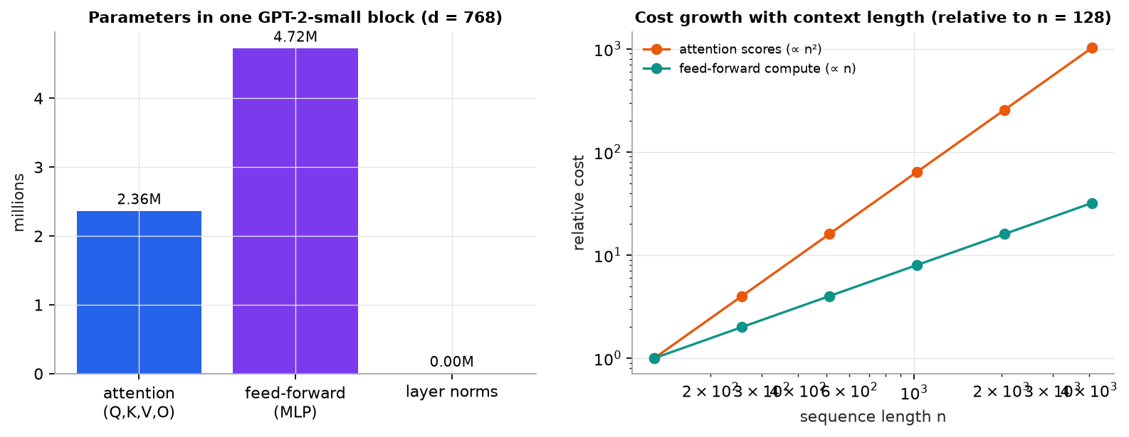
The feed-forward network holds about two-thirds of each block's parameters. Attention's score matrix is what grows quadratically with context.
Interactive: step through self-attention, the core of each block, with shapes. Open the lab.
3. The math
Symbols
| Symbol | Meaning |
|---|---|
| the sequence of token representations, shape | |
| model width () | |
| feed-forward hidden width, typically | |
| number of attention heads | |
| number of blocks | |
| vocabulary size |
A pre-norm block
Shapes never change through a block: in, out. That is what makes blocks stackable.
Positional information
Attention treats its input as a set: shuffle the tokens and each output row is shuffled the same way, with nothing else changed. Order has to be injected. Three schemes matter:
- Learned absolute (GPT-2): a trainable table
pos_embof shape , added to the token embedding. Nothing exists pastctx. - Sinusoidal (original transformer): a fixed table, no parameters. For position and feature pair :
With at : pair has frequency , giving and . Pair has frequency , giving and . Low pairs spin fast and tell neighbours apart; high pairs spin slowly and encode coarse position.
- Rotary (RoPE), used by most current open LLMs: instead of adding anything, rotate each pair of query and key features by an angle proportional to the position. Rotating by angle and by angle makes depend only on the offset , so attention sees relative distance directly.
Families
| Family | Attention pattern | Typical use | Examples |
|---|---|---|---|
| Encoder-only | bidirectional (no mask) | classification, embeddings, extraction | BERT-style encoders, embedding models |
| Decoder-only | causal mask | text generation, chat LLMs | GPT-style models |
| Encoder-decoder | encoder bidirectional; decoder causal plus cross-attention to the encoder's outputs | translation, summarization | T5-style models |
In cross-attention, queries come from the decoder and keys and values from the encoder, so each generated token can look at the whole input.
Worked example: counting GPT-2-small's parameters
, , , , context 1,024.
- Attention per block: are each with biases: .
- Feed-forward per block: .
- Layer norms per block: two, each with scale and shift: .
- Block total: . Twelve blocks: .
- Embeddings: tokens plus positions , total . The output head reuses the token embedding (weight tying).
- Final layer norm: .
Total: , the published 124M.
Compute per token
A forward pass costs roughly multiply-adds per token, plus the attention-score term that grows with context length (about per layer per token).
4. Implementation
The full script is code/14-transformers/gpt_scratch.py (NumPy only). It reuses attention, softmax, and split_heads from the self-attention lesson's script and assembles a complete GPT-style forward pass.
Build it from scratch
Step 1: one shape table for the whole model. Every parameter's shape is written down once. The same table initializes the tiny model and counts GPT-2-small, so the count in section 3 is checked by code rather than trusted. The query, key, and value projections are fused into one matrix, as in GPT-2.
def param_shapes(V, ctx, d, L, d_ff):
    block = {"ln1_g": (d,), "ln1_b": (d,), "W_qkv": (d, 3 * d), "b_qkv": (3 * d,),
             "W_o": (d, d), "b_o": (d,), "ln2_g": (d,), "ln2_b": (d,),
             "W_1": (d, d_ff), "b_1": (d_ff,), "W_2": (d_ff, d), "b_2": (d,)}
    top = {"tok_emb": (V, d), "pos_emb": (ctx, d), "lnf_g": (d,), "lnf_b": (d,)}
    return top, [block] * L          # no separate output head: it reuses tok_emb
Predict: if you untie the output head (add a separate (d, V) matrix), how many parameters does GPT-2-small gain?
Step 2: the per-token operations. LayerNorm normalizes each token's features to mean 0 and variance 1, then rescales with learned g and b. The MLP widens each token to , applies GELU, and projects back. Neither looks at other tokens.
def layer_norm(x, g, b, eps=1e-5):
    mu = x.mean(axis=-1, keepdims=True)                  # per token, over the d features
    var = x.var(axis=-1, keepdims=True)
    return g * (x - mu) / np.sqrt(var + eps) + b

def gelu(x):                                             # tanh approximation used by GPT-2
    return 0.5 * x * (1 + np.tanh(np.sqrt(2 / np.pi) * (x + 0.044715 * x ** 3)))

def mlp(x, p):
    return gelu(x @ p["W_1"] + p["b_1"]) @ p["W_2"] + p["b_2"]   # [n, d] -> [n, d_ff] -> [n, d]
Predict: LayerNorm here uses axis=-1. What would go wrong at inference if it normalized over the sequence axis instead?
Step 3: causal multi-head attention. One matrix multiply produces Q, K, and V side by side; np.split cuts them apart. Then it is the batched multi-head attention from the previous lesson, followed by the output projection.
def causal_mha(x, p, h):
    q, k, v = np.split(x @ p["W_qkv"] + p["b_qkv"], 3, axis=-1)   # three [n, d]
    out, _ = attention(split_heads(q, h), split_heads(k, h), split_heads(v, h), causal=True)
    merged = out.transpose(1, 0, 2).reshape(x.shape[0], -1)       # [n, d]
    return merged @ p["W_o"] + p["b_o"]
Predict: attention is the only place tokens exchange information. If you removed the causal mask here, which check in the output below would fail?
Step 4: one pre-norm block. This is the two-line formula from section 3. Each sublayer sees a normalized copy of x, and its output is added to x. The residual path itself is never normalized, which is why gradients reach early layers cleanly.
def block(x, p, h):
    x = x + causal_mha(layer_norm(x, p["ln1_g"], p["ln1_b"]), p, h)   # communicate
    x = x + mlp(layer_norm(x, p["ln2_g"], p["ln2_b"]), p)             # compute
    return x                                                          # still [n, d]
Predict: if every weight in a block were zero, what would the block output?
Step 5: the whole model. Look up a token vector and a position vector and add them. Run the blocks, apply a final LayerNorm, and multiply by the transposed token embedding to get one logit per vocabulary entry at every position.
def gpt_forward(ids, P, h):
    n = len(ids)
    x = P["tok_emb"][ids] + P["pos_emb"][:n]           # [n, d]: what + where
    for p in P["blocks"]:
        x = block(x, p, h)
    x = layer_norm(x, P["lnf_g"], P["lnf_b"])
    return x @ P["tok_emb"].T                          # tied head: logits [n, V]
Predict: generation only needs the logits at the last position. What fraction of this computation does a KV cache let you skip for each new token?
Use the library
The PyTorch block below is the same computation as steps 2 to 4, with autograd, dropout, and fused GPU kernels. nn.MultiheadAttention holds separate Q, K, V weights where GPT-2 fuses them, but the parameter count is identical.
import torch
from torch import nn

class Block(nn.Module):
    def __init__(self, d=768, heads=12, d_ff=3072, dropout=0.1):
        super().__init__()
        self.ln1, self.ln2 = nn.LayerNorm(d), nn.LayerNorm(d)
        self.attn = nn.MultiheadAttention(d, heads, dropout=dropout, batch_first=True)
        self.ff = nn.Sequential(nn.Linear(d, d_ff), nn.GELU(), nn.Linear(d_ff, d), nn.Dropout(dropout))

    def forward(self, x):                                  # x: [B, n, d]
        n = x.size(1)
        causal = torch.triu(torch.ones(n, n, dtype=torch.bool, device=x.device), diagonal=1)
        h = self.ln1(x)
        x = x + self.attn(h, h, h, attn_mask=causal, need_weights=False)[0]   # residual 1
        return x + self.ff(self.ln2(x))                                       # residual 2

print(sum(p.numel() for p in Block().parameters()))       # 7,087,872
To load real GPT-2 weights instead of random ones, use Hugging Face transformers (AutoModelForCausalLM.from_pretrained("gpt2")).
Run it
uv run code/14-transformers/gpt_scratch.pyKey lines of the output (the tiny model's weights are synthetic and random):
== GPT-2-small parameter count from the shape table ==
total: 124,439,808
one block: 7,087,872
ids shape: (5,) -> logits shape: (5, 12)
positions 0-3 unchanged: True
position 4 changed:      True
sequence: [3, 7, 1, 4, 9, 9, 9, 9, 9, 9]
The totals match the hand count in section 3. Changing the last token leaves earlier logits untouched, which proves the mask works. Random weights generate a repeated token, which is what an untrained model does. FLOP and memory figures are in code/15-llms/llms.py.
5. Engineering
Scaling. Model quality improves predictably with parameters, data, and compute (scaling laws). Width and depth grow together; modern models add tweaks such as RMSNorm instead of LayerNorm, SwiGLU feed-forward layers, rotary position embeddings, and grouped-query attention to cut KV-cache memory.
Memory and latency. Weights dominate memory for short contexts; the KV cache dominates for long contexts and large batches. Attention cost grows with during prefill (processing the prompt); each new generated token costs with a KV cache.
Choosing a family. Use encoder models for classification, retrieval embeddings, and token tagging (cheaper, bidirectional). Use decoder models for open-ended generation and instruction following. Encoder-decoders remain strong for translation and structured transformation tasks.
Watch outFailure modes. Missing or wrong causal masks; position handling that breaks beyond the trained context length; numerical instability in deep post-norm stacks; underestimating KV-cache memory when raising batch size or context.
Common mistakes
- Assuming attention holds most of the parameters (the feed-forward layers do).
- Forgetting weight tying when counting parameters.
- Using a decoder-only model where a small encoder would do the job cheaper.
6. Knowledge check
Quiz: The transformer architecture
How many parameters (with biases) does a feed-forward sublayer have with and ?
Practice exercise. Count the parameters of one block with and (with biases and two layer norms).
Solution
Attention: . FFN: . Layer norms: . Total: .
Implementation challenge. Stack 4 Blocks with token and position embeddings and a tied output head, train it on a small text file for next-character prediction, and sample from it.
Summary
- A block is attention (communication) plus a feed-forward network (per-token computation), each with a residual connection and layer normalization.
- Shapes stay through every block, so blocks stack.
- The feed-forward layers hold about two-thirds of block parameters; GPT-2 small totals 124M.
- Encoder-only for understanding and embeddings, decoder-only for generation, encoder-decoder (with cross-attention) for sequence-to-sequence tasks.
Next: BERT and masked language modeling
Related: Self-attention · Model card: transformer encoder · Model card: transformer decoder
Go deeper, code-first (AI Engineering from Scratch): Machine Translation
Parts of this lesson are adapted from AI Engineering from Scratch by Rohit Ghumare (MIT license, notice): Positional Encoding — Sinusoidal, RoPE, ALiBi, The Full Transformer — Encoder + Decoder, Build a Transformer from Scratch — The Capstone, Token and Positional Embeddings, Transformer Block from Scratch, GPT Model Assembly.
Interview angle
Why do residual connections help deep networks train?
They give both the signal and the gradient an identity path around every block. A residual block computes , so . When gradients flow back through blocks, the product of these Jacobians always contains the identity term, so the gradient can't shrink to zero just because some are small. Without residuals, the gradient is a product of factors that tends to vanish or explode. Residuals also change what each block learns: only a change to the representation, and at initialization, when is near zero, the whole network is close to the identity, an easy starting point. In transformers the residual stream carries information through all layers while attention and the FFN read from and write to it. Pre-norm, , keeps that identity path clean, which is why it trains stably in deep stacks.
For ticket classification and semantic search, would you use an encoder-only or a decoder-only model?
Usually an encoder-only model, at least as the first baseline. Encoders attend bidirectionally, so every token's representation uses context on both sides, which is what you want for classification, token tagging, and embeddings. They are small (100M to 400M parameters is common), so they are cheap to fine-tune and serve, and a forward pass gives you the answer with no generation loop. For semantic search, a bi-encoder produces one vector per document for a vector index. A decoder-only LLM can classify zero-shot or few-shot with no labeled data and handles open-ended outputs, but it costs far more per request and adds latency from autoregressive decoding. My order: with labeled data, fine-tune a small encoder; without it, prompt a decoder model to bootstrap labels, then distill into an encoder if volume makes the cost matter. Encoder-decoders fit sequence-to-sequence tasks such as translation.
Estimate the parameter count and per-token compute of a decoder with d = 4096, 32 layers, d_ff = 4d, and a 32,000-token vocabulary.
About 6.6 billion parameters and about 13 GFLOPs per token. Per block, attention has weights () and the FFN has , so a block is about ; biases and layer norms are negligible. Thirty-two blocks give about . The token embedding adds , and an untied output head adds the same again. Total is about 6.6 to 6.7 billion, a "7B-class" model. LLaMA-style models use a SwiGLU FFN with three matrices and , which keeps the FFN near . A forward pass costs about parameters FLOPs per token, about 13 GFLOPs, plus an attention term that grows with context. Two-thirds of the block parameters live in the FFN.
Your model works well up to 4,000 tokens, but quality collapses on longer inputs. What is going on?
Most likely the model was trained at a 4,096-token context and position handling doesn't extrapolate. Learned absolute position embeddings simply don't exist past the trained length. Rotary embeddings (RoPE) produce rotation angles at long positions the model never saw, and attention patterns break down. Check the training context length in the model config first. Then rule out pipeline bugs: silent truncation by the tokenizer or server, a wrong max_position_embeddings, or a chat template that pushes the instructions out of the window. If it really is extrapolation, the fixes are RoPE scaling methods such as position interpolation, which compress positions into the trained range and usually need a short fine-tune on long sequences, or switching to a model trained for long context. Even within the trained window, measure retrieval of facts placed in the middle of long inputs; models often attend to them less reliably.