Training and regularization

Quick read: the intuition, interactive visualization, summary, and interview questions. The math, implementation, engineering, and knowledge-check sections are hidden.

Mental model. A large network can memorize its training set. Regularization makes memorizing harder than learning the general pattern, and validation loss tells you whether it is working. Training loss tells you how well the model fits; validation loss tells you how well it generalizes.

You will learn to

Diagnose training from training and validation curves and choose an early-stopping point.
Apply weight decay (L2), L1, dropout, batch and layer normalization, and data augmentation, and say what each does.
Choose a learning-rate schedule, including warmup.
Run grid search, random search, and Bayesian optimization, with cross-validation where appropriate.

Why it matters. Most of the gap between a model that "works on my machine" and one that generalizes is training discipline. These are also the knobs you will tune most often in practice.

1. Intuition

Plot loss after every epoch on the training and validation sets. Early on, both fall. Eventually training loss keeps falling while validation loss stops improving and starts rising: the model has begun fitting noise in the training set. The best model is the one at the validation minimum, which is what early stopping keeps.

Regularization techniques push in the same direction in different ways:

Weight decay (L2): penalizes large weights, favoring smoother functions.
Dropout: randomly zeroes a fraction of activations during training, so the network can't rely on any single unit and learns redundant, robust features. It is switched off at inference.
Normalization (batch norm, layer norm): rescales activations to a stable range, which speeds training and has a mild regularizing effect.
Data augmentation: creates label-preserving variations (flipped or cropped images, noise, paraphrases) so the model sees more diverse examples.

The learning rate changes over training: often a short warmup from near zero (stabilizes early updates, especially for transformers), then a decay so the model settles into a minimum instead of bouncing around it.

2. Visualization

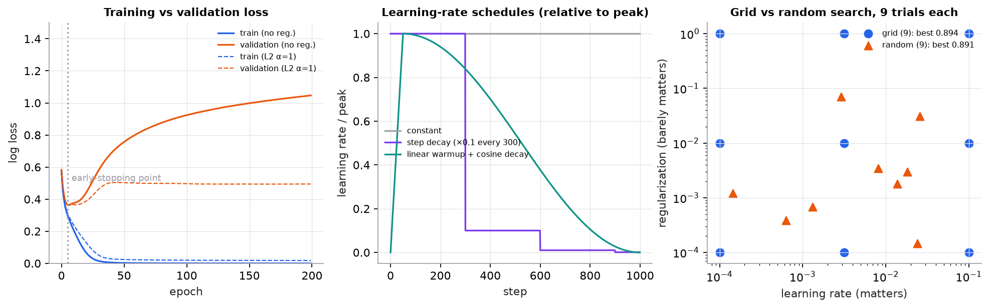
Synthetic classification task, MLP with two hidden layers of 256 units. Search panel uses a synthetic validation surface on which only the learning rate matters much.

3. The math

Symbols

Symbol	Meaning
$L_{\text{data}}$	the training loss (e.g. cross-entropy)
$\lambda$	regularization strength
$p$	dropout probability (fraction of units zeroed)
$\mu_B, \sigma_B^2$	mean and variance of a batch (batch norm)
$\gamma, \beta$	learnable scale and shift in normalization layers
$\eta_t$	learning rate at step $t$

Weight decay and L1

L = L_{\text{data}} + \lambda\sum_j w_j^2 \quad (\text{L2}) \qquad L = L_{\text{data}} + \lambda\sum_j |w_j| \quad (\text{L1})

With plain SGD, the L2 term adds $2\lambda w$ to the gradient, so each step shrinks weights by a constant factor ("decay"). With Adam this equivalence breaks, which is why AdamW applies decay directly to the weights.

Dropout

During training, each activation is kept with probability $1 - p$ and scaled by $\frac{1}{1-p}$ so its expected value is unchanged:

\tilde{a}_i = \frac{m_i}{1 - p}\,a_i, \qquad m_i \sim \text{Bernoulli}(1 - p)

At inference all units are kept and no scaling is applied.

Normalization

\hat{a} = \frac{a - \mu}{\sqrt{\sigma^2 + \epsilon}}, \qquad \text{output} = \gamma\,\hat{a} + \beta

Batch norm computes $\mu, \sigma^2$ per feature across the batch (and uses running averages at inference). Layer norm computes them per example across features, which doesn't depend on batch size, so it is the standard in transformers.

Cosine schedule with warmup

\eta_t = \begin{cases} \eta_{\max}\,\dfrac{t}{T_w} & t < T_w \\[4pt] \dfrac{\eta_{\max}}{2}\left(1 + \cos\dfrac{\pi(t - T_w)}{T - T_w}\right) & t \ge T_w \end{cases}

Worked example 1: dropout scaling

A layer's activations are $[2, 4, 6, 8]$ with $p = 0.5$ . A sampled mask is $[1, 0, 1, 0]$ . Kept units are scaled by $1/(1 - 0.5) = 2$ : output $[4, 0, 12, 0]$ . The mean of the original activations is 5; the expected value of each scaled output equals its original value, so on average the next layer sees the same scale at training and inference.

Worked example 2: layer norm

Activations $a = [1, 2, 3, 6]$ . Mean $\mu = 3$ ; variance $\sigma^2 = \frac{4 + 1 + 0 + 9}{4} = 3.5$ ; standard deviation $1.871$ . Normalized: $[-1.069, -0.535, 0, 1.604]$ . With $\gamma = 1$ , $\beta = 0$ that is the output.

Worked example 3: reading the curves

Without regularization, validation loss reached its minimum (0.364) at epoch 6 and climbed to 1.047 by epoch 200, while training loss kept falling. Early stopping with patience would have kept the epoch-6 weights. With L2 strength 1.0, the best validation loss was similar (0.362), but the final value was 0.495: regularization made the model far less sensitive to training too long.

4. Implementation

The full script is code/12-training-regularization/training_scratch.py (NumPy only). It builds the five tools a training loop leans on, each in a few lines, and checks them against the worked examples above.

Build it from scratch

Step 1: inverted dropout. Draw a keep-mask, zero the dropped units, and scale the survivors by $1/(1-p)$ during training. Because the scaling happens at training time, inference needs no change at all: the layer just returns its input.

python

def dropout(a, p, rng, training=True):
    if not training or p == 0:
        return a                                  # inference: identity, no rescaling
    mask = rng.random(a.shape) >= p               # keep with probability 1 - p
    return a * mask / (1 - p)

Predict: average this function's output over many random masks. What do you get for the input [2, 4, 6, 8]?

Step 2: layer norm. Mean and variance per example, across features (axis=-1), so the result never depends on the other examples in the batch. That is why it works at batch size 1 and is the default in transformers.

python

def layer_norm(a, gamma=1.0, beta=0.0, eps=1e-5):
    mu = a.mean(axis=-1, keepdims=True)
    var = a.var(axis=-1, keepdims=True)           # population variance (divide by n)
    return gamma * (a - mu) / np.sqrt(var + eps) + beta

Predict: change axis=-1 to axis=0 and you have batch norm's training-time statistics. What goes wrong at inference with a batch of one?

Step 3: initialization. Each layer multiplies the signal's variance by about fan_in * std**2 (halved again by ReLU, which zeros half its inputs). Set std so that product is 1 and the signal keeps its scale through depth. Too small and it shrinks geometrically to zero; too large and it explodes.

python

def init(fan_in, fan_out, scheme, rng):
    std = {"small": 0.01,
           "xavier": math.sqrt(1 / fan_in),       # LeCun/Xavier-style, for tanh
           "he": math.sqrt(2 / fan_in)}[scheme]   # ReLU zeros half the inputs, so double it
    return rng.normal(0, std, (fan_in, fan_out))

Predict: with width 256 and std = 0.01, each layer multiplies the variance by $256 \times 0.0001 = 0.0256$ . Roughly how small is the standard deviation after 10 layers? (Here fan_in = fan_out, so Xavier's $2/(\text{fan\_in} + \text{fan\_out})$ equals $1/\text{fan\_in}$ .)

Step 4: warmup plus cosine. The formula from section 3, plus a floor min_lr. Warmup keeps the first steps small while Adam's moment estimates and the early activations settle; the cosine then decays smoothly to the floor.

python

def lr_at(t, max_lr, warmup, total, min_lr=0.0):
    if t < warmup:
        return max_lr * (t + 1) / warmup          # ramp up from max_lr/warmup to max_lr
    progress = (t - warmup) / max(1, total - warmup)
    return min_lr + 0.5 * (max_lr - min_lr) * (1 + math.cos(math.pi * progress))

Predict: halfway through the decay phase, progress = 0.5. What fraction of the way from max_lr down to min_lr is the rate?

Step 5: early stopping. Track the best validation loss and its epoch. Stop after patience epochs without improvement, and restore the best epoch's weights, not the last ones.

python

def early_stop(val_losses, patience):
    best, best_epoch, bad = float("inf"), -1, 0
    for epoch, v in enumerate(val_losses):
        if v < best:
            best, best_epoch, bad = v, epoch, 0   # new best: this is the checkpoint to keep
        else:
            bad += 1
            if bad >= patience:
                return best_epoch, epoch          # stopped here, restore best_epoch
    return best_epoch, len(val_losses) - 1

Predict: with a noisy validation curve, does a larger patience make you stop earlier or later, and what does it cost?

Use the library

In PyTorch each tool is one line: nn.Dropout (step 1, switched by model.train() and model.eval()), nn.LayerNorm (step 2), nn.init.kaiming_normal_ and xavier_normal_ (step 3; nn.Linear already uses a scaled uniform init by default), a scheduler (step 4), and the patience loop (step 5). OneCycleLR below ramps up for the first 30% of steps and then anneals (both phases cosine-shaped by default); for warmup-then-cosine with a separate floor, chain LinearLR and CosineAnnealingLR with SequentialLR.

python

import torch
from torch import nn

model = nn.Sequential(
    nn.Linear(40, 256), nn.LayerNorm(256), nn.ReLU(), nn.Dropout(p=0.3),
    nn.Linear(256, 256), nn.LayerNorm(256), nn.ReLU(), nn.Dropout(p=0.3),
    nn.Linear(256, 1),
)
opt = torch.optim.AdamW(model.parameters(), lr=1e-3, weight_decay=0.01)
sched = torch.optim.lr_scheduler.OneCycleLR(opt, max_lr=1e-3, total_steps=epochs * len(train_loader))

best, patience, bad = float("inf"), 10, 0
for epoch in range(epochs):
    model.train()                                  # dropout ON
    for xb, yb in train_loader:
        opt.zero_grad()
        loss = nn.functional.binary_cross_entropy_with_logits(model(xb).squeeze(-1), yb)
        loss.backward()
        torch.nn.utils.clip_grad_norm_(model.parameters(), 1.0)
        opt.step(); sched.step()
    model.eval()                                   # dropout OFF
    with torch.no_grad():
        val = evaluate(model, val_loader)
    if val < best:
        best, bad = val, 0
        torch.save(model.state_dict(), "best.pt")  # keep the best checkpoint
    else:
        bad += 1
        if bad >= patience:
            break                                  # early stopping

Hyperparameter search with scikit-learn:

python

from scipy.stats import loguniform
from sklearn.model_selection import RandomizedSearchCV
search = RandomizedSearchCV(estimator, {"alpha": loguniform(1e-5, 1), "learning_rate_init": loguniform(1e-4, 1e-1)},
                            n_iter=30, cv=5, random_state=0)

Run it

bash

uv run code/12-training-regularization/training_scratch.py

Key lines of the output (the activations and validation curve are synthetic):

text

scaled output: [ 4.  0. 12.  0.]
mean over 100,000 random masks: [2.005 3.989 5.965 8.003]  (original: [2. 4. 6. 8.] )
[-1.069 -0.535  0.     1.604]
 std 0.01 + tanh: 1.56e-01  1.02e-04  1.08e-08  1.14e-16
       he + relu: 8.27e-01  8.59e-01  8.87e-01  1.05e+00
   xavier + relu: 5.85e-01  1.52e-01  2.77e-02  1.03e-03
step  550: lr = 1.650e-04
best epoch 6 (val 0.364), stopped at epoch 11

The first three lines match worked examples 1 and 2. The init rows are the standard deviation after layers 1, 5, 10, and 20: a tiny fixed scale vanishes, He keeps ReLU activations near 1, and Xavier (designed for tanh) loses about half the variance per ReLU layer. The real training curves, schedules, and search comparison are in code/11-gradient-descent-backprop/backprop_training.py.

5. Engineering

Hyperparameter search. Grid search tries every combination on a fixed grid; random search samples combinations at random. When only a few hyperparameters really matter, random search explores more distinct values of each one for the same budget: in the figure's 9 trials, grid tried 3 learning rates and random tried 9. (On this particular run grid search still scored slightly higher, 0.894 versus 0.891, because its grid happened to land near the optimum. The advantage is in coverage, not a guarantee every time.) Bayesian optimization (Optuna, scikit-optimize) models the validation score and proposes promising settings, which is better for expensive training runs. Search learning rates and regularization strengths on a log scale.

Cross-validation is affordable for classical models and small networks; for large deep models, a single fixed validation split is the norm.

What to tune first: learning rate, then model size and regularization (weight decay, dropout), then batch size and schedule.

Reproducibility: seed everything, log configurations and metrics (an experiment tracker helps), and save the best checkpoint, not the last.

Watch out
Failure modes. Selecting hyperparameters on the test set; forgetting model.eval() so dropout and batch norm behave like training at inference; batch norm with tiny batches; augmentation that changes the label (flipping a "6" into a "9"); stopping on a noisy validation curve without patience.

Common mistakes

Using L2 penalty with Adam and expecting weight decay (use AdamW).
Evaluating a model while it is still in training mode.
Leaving initialization to chance in a custom layer. A weight scale that is slightly too small shrinks activations geometrically with depth (std 0.01 at width 256 leaves about 1e-8 after 10 tanh layers); use He init for ReLU and Xavier for tanh, or rely on the framework defaults plus normalization.
Reporting the last epoch's validation score instead of the best checkpoint's (or reporting the best checkpoint's validation score as if it were a test score).

6. Knowledge check

Quiz: Training and regularization

Question 1 of 6

Fill inmedium

Activations [2, 6, 4], dropout $p = 0.5$ , mask [0, 1, 1]. What is the training-time output? Answer like [a, b, c].

Practice exercise. Activations $[3, 1, 4, 2]$ pass through dropout with $p = 0.25$ and mask $[1, 1, 0, 1]$ . What is the output? Then compute layer norm of $[3, 1, 4, 2]$ (with $\gamma = 1$ , $\beta = 0$ ).

Solution

Scale is $1/0.75 = 1.333$ : output $[4, 1.333, 0, 2.667]$ . Layer norm: mean 2.5, variance $\frac{0.25 + 2.25 + 2.25 + 0.25}{4} = 1.25$ , std 1.118. Output $[0.447, -1.342, 1.342, -0.447]$ .

Implementation challenge. Train the same MLP on a small dataset four ways (no regularization, weight decay, dropout, both), plot all training and validation curves on one figure, and report the best validation loss and the epoch where it occurred for each.

Summary

Watch training and validation loss together; keep the checkpoint at the validation minimum (early stopping).
Weight decay, dropout, normalization, and augmentation each make memorization harder.
Warmup plus decay schedules stabilize early training and help the model settle.
Tune on validation data, prefer random or Bayesian search on log scales, and never tune on the test set.

Next: Debugging neural networks

Parts of this lesson are adapted from AI Engineering from Scratch by Rohit Ghumare (MIT license, notice): Regularization, Weight Initialization and Training Stability, Learning Rate Schedules and Warmup, Cosine LR with Linear Warmup.

Interview angle

How does dropout work, and why do you scale the kept activations by 1/(1−p)?

During training, dropout zeroes each activation independently with probability $p$ and multiplies the survivors by $1/(1-p)$ ; at inference it does nothing. The scaling keeps the expected activation unchanged, so the next layer sees the same scale in training and inference: $E[\tilde{a}] = (1-p) \cdot a/(1-p) = a$ . In the course example, $[2, 4, 6, 8]$ with $p = 0.5$ and mask $[1, 0, 1, 0]$ becomes $[4, 0, 12, 0]$ . Because any unit can disappear, the network can't rely on a single co-adapted feature and learns redundant ones. One view is that it trains an ensemble of thinned subnetworks that share weights and averages them at test time. Practical points: forgetting model.eval() leaves dropout on at inference and gives noisy predictions, and large pretrained transformers often use little or no dropout because their data is large relative to their capacity.

Batch norm versus layer norm: why do transformers use layer norm?

Batch norm normalizes each feature using the mean and variance across the batch; layer norm normalizes each example across its own features. Batch norm's dependence on the batch causes problems for transformers: statistics are noisy with small per-device batches, sequences have variable lengths and padding, and inference must use running averages, which creates a train/inference mismatch and makes autoregressive decoding one token at a time awkward. Layer norm computes everything per example, so it behaves the same at any batch size and in training and inference. For $[1, 2, 3, 6]$ : mean 3, variance 3.5, output $[-1.069, -0.535, 0, 1.604]$ . Batch norm is still a strong choice for CNNs with large batches, where its batch noise also acts as a mild regularizer. Many modern LLMs use RMSNorm, which drops the mean subtraction and is slightly cheaper.

Training loss keeps falling, but validation loss bottoms out at epoch 6 and climbs after that. What do you do?

That is classic overfitting, but confirm it before treating it. Check that validation data comes from the same distribution as training and that no leakage or preprocessing difference explains the gap. Also check accuracy alongside loss: if validation loss rises while accuracy stays flat, the model is becoming overconfident on its mistakes, which matters if you use its probabilities. Then act: keep the epoch-6 checkpoint with early stopping and a patience of several epochs so noise doesn't stop you too soon; add weight decay (with AdamW), dropout, or data augmentation that preserves labels; reduce model size or get more data. In the course's synthetic run, validation loss hit its minimum of 0.364 at epoch 6 and climbed to about 1.05 by epoch 200, while L2 regularization flattened that rise. Report the selected checkpoint's score on a held-out test set, not its validation score.

You have budget for 20 training runs to tune learning rate, weight decay, and dropout. How do you spend it?

Random search on log scales, with learning rate prioritized, not a grid. A $3 \times 3 \times 2$ grid of 18 runs tries only three learning rates; 20 random samples try 20 distinct values of each hyperparameter. Since one or two hyperparameters usually dominate (often learning rate), random search explores the important axis far better. Sample learning rate log-uniformly over, say, $10^{-4}$ to $10^{-2}$ , weight decay log-uniformly over $10^{-5}$ to $10^{-1}$ , and dropout uniformly over 0 to 0.5. Use early stopping or successive halving to kill bad runs early, which stretches the budget further. With leftover runs, narrow the range around the best region or switch to Bayesian optimization. Select on validation or cross-validation, re-run the winner with two or three seeds to check it wasn't luck, and touch the test set once at the end.