Module 12: Training and regularization 45 min10 min quick readDeep learning
Debugging neural networks
Find silent training bugs in a fixed order (initial loss, gradient check, overfit one batch, per-layer statistics, learning-rate sweep) and map each symptom to its likely cause and first fix.
Before this: Training and regularization, Intro to PyTorch, Numerical stability
Quick read: the intuition, interactive visualization, summary, and interview questions. The math, implementation, engineering, and knowledge-check sections are hidden.
Mental model. A broken network rarely crashes. It runs, prints a loss, and quietly learns the wrong thing. So you debug it like a doctor, not like a compiler: take cheap vital signs in a fixed order (does the first loss make sense, do gradients match, can it memorize one batch, is every layer alive), and only then reach for expensive tests.
You will learn to
- Predict the loss at step 0 and use it to catch bad initialization and label bugs.
- Run a gradient check and an overfit-one-batch test, and say what each one rules out.
- Read per-layer statistics (dead-unit fraction, gradient norm, update-to-weight ratio) to find dead or vanishing layers.
- Use a learning-rate range test to pick a starting learning rate.
- Map a symptom (NaN, flat loss, chance accuracy, train/val gap) to its likely cause and first fix.
Why it matters. "My loss isn't going down, what do you do?" is one of the most common practical interview questions, because the answer shows whether you can work without an error message. In real projects, a misaligned label or a missing line wastes days of GPU time. Most of these bugs can be caught in the first minute of training if you know where to look.
1. Intuition
Ordinary bugs announce themselves: an exception, a wrong number in a unit test. Neural-network bugs mostly don't. A transposed dimension broadcasts silently. Shuffled labels still give a loss that decreases a little. A dead layer still outputs zeros that the next layer happily uses.
So build confidence from the bottom up, cheapest checks first:
- Look at the data. Plot a few inputs with their labels. Check that labels line up with inputs and that inputs are normalized.
- Check the loss at step 0. A fresh classifier should be unsure of everything, so its loss should be close to that of a uniform guess, for classes. Far above means it is confidently wrong before learning; far below means something leaks the answer.
- Check gradients against finite differences when you write any backward pass yourself.
- Overfit one small batch. A correct model and training loop can memorize 16 examples to near-zero loss. If it can't, nothing about data size or regularization matters yet: the plumbing is broken.
- Watch every layer. Fraction of units that never activate, gradient size per layer, and how big each update is compared with the weights.
- Sweep the learning rate once, quickly, instead of guessing.
Only after all of that do you scale up and start worrying about generalization, which is the previous lesson's subject.
2. Visualization
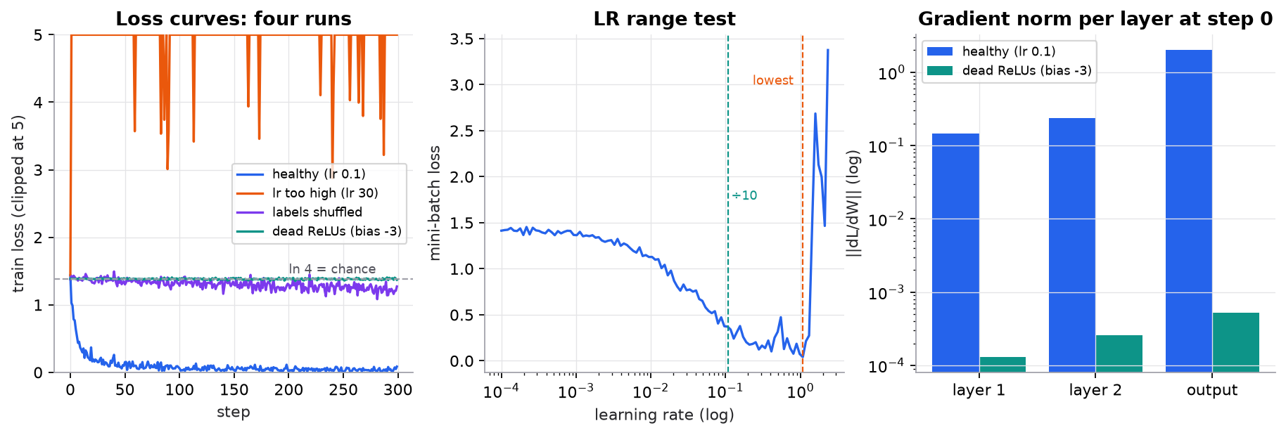
Synthetic data: 800 points in 10 dimensions from 4 Gaussian blobs. Left: three different bugs, two of which look identical on the loss curve. Middle: one sweep finds the usable learning-rate range. Right: the per-layer view tells the dead-ReLU bug apart from the shuffled-label bug, which the loss curve alone cannot.
Try it (predict, then run the script):
- In the left panel, shuffled labels and dead ReLUs both stall near chance. Which diagnostic from the script would you run to tell them apart, and what would each show?
- Change the dead-ReLU bias from −3 to −1. Predict whether the network recovers.
- In the LR range test, the loss keeps falling until about 1. Why is the suggestion one tenth of that rather than the minimum itself?
- Set
out_scale=1.0ininit()and rerun the healthy model. Predict the step-0 loss and whether the model still trains.
3. The math
Symbols
| Symbol | Meaning | Shape |
|---|---|---|
| number of classes | integer | |
| loss at step 0 | scalar | |
| weight matrix of layer | ||
| gradient of the loss with respect to | same as | |
| Frobenius norm (square root of the sum of squares) | scalar | |
| learning rate | scalar | |
| finite-difference step | scalar |
Check 1: the step-0 loss
If the model predicts uniform probabilities , cross-entropy is
| 2 | 4 | 10 | 1,000 | 50,000 (a token vocabulary) | |
|---|---|---|---|---|---|
| 0.693 | 1.386 | 2.303 | 6.908 | 10.820 |
In the script, : He initialization with a small (×0.1) output layer gives 1.421, close to 1.386. He init everywhere gives 2.336: the logits start large enough that the model is already somewhat confident. Weights with standard deviation 3.0 give 1705.6: the true class gets a probability of about , and the first updates will be huge.
Check 2: gradient check
For a weight entry :
Use float64 and (see numerical stability). Below about passes (ReLU kinks can add a little noise); around or more is a bug. The script's correct backward gives . Forgetting to multiply by the ReLU mask in backward gives : the gradient is simply wrong.
Check 3: overfit one batch
On 16 examples, full-batch gradient descent should drive the loss toward 0. The script goes (step 100) (step 300), with 100% batch accuracy. A model that can't do this has a bug in the loss, the backward pass, the optimizer wiring (for example an optimizer built over the wrong parameters), or the input/label pairing.
Check 4: update-to-weight ratio
This is the fraction by which one plain-SGD step changes the layer's weights. A widely used heuristic for hidden layers is around : much larger (above ) and the layer is thrashing; much smaller (below ) and it is barely moving. It is a rule of thumb, not a law; adaptive optimizers and the first few steps vary.
Worked example. Layer 1 maps 10 inputs to 32 units with He init, standard deviation . Its norm is about (the script's actual draw is 8.18). The script measures at step 0. With :
Right in the healthy range. The dead-ReLU network has , giving : a thousand times too small to learn in any reasonable time. (The output layer's ratio is large at step 0, 0.66, only because its weights were initialized 10 times smaller on purpose.)
Check 5: dead units
A ReLU unit is dead on a batch if its pre-activation is for every example, so it outputs 0 and passes back zero gradient. With a hidden bias of , layer 1's pre-activations (before the bias) have a standard deviation of about 2.3, so each unit clears the −3 bias on only about 9% of examples; just 3% of units are dead on all 64. Layer 2 then receives mostly zeros, its pre-activations sit near , and 97% of its units are dead. Gradients through it are near zero, and the loss stalls at .
4. Implementation
Build it from scratch
The model is a two-hidden-layer MLP in NumPy, with the forward pass keeping every activation for the backward pass and the diagnostics. init uses He scaling for ReLU layers and shrinks the output layer so the step-0 loss starts near .
def init(seed=0, w_scale=None, b_hidden=0.0, out_scale=0.1):
    rng = np.random.default_rng(seed)
    sizes = [D, H, H, K]
    params = []
    for i, (a, b) in enumerate(zip(sizes, sizes[1:])):
        s = w_scale if w_scale is not None else math.sqrt(2 / a)        # He init for ReLU layers
        if i == len(sizes) - 2 and w_scale is None:
            s *= out_scale                                              # small output layer: near-uniform start
        bias = np.full(b, b_hidden if i < 2 else 0.0)
        params.append([rng.normal(0, s, (a, b)), bias])
    return params
Predict: with out_scale=0.0, what is the step-0 loss exactly? (All logits equal the output bias, 0, so it's exactly .)
The backward pass is where bugs hide. The relu_mask_bug flag lets us plant one on purpose: leaving out the ReLU mask passes gradient through units that were off.
def loss_and_grads(params, X, y, relu_mask_bug=False):
    acts = forward(params, X)
    z = acts[-1]
    z = z - z.max(1, keepdims=True)
    logp = z - np.log(np.exp(z).sum(1, keepdims=True))
    loss = -logp[np.arange(len(y)), y].mean()
    d = np.exp(logp)
    d[np.arange(len(y)), y] -= 1
    d /= len(y)                                                         # dL/dlogits = (softmax - onehot) / n
    grads = [None] * len(params)
    for i in reversed(range(len(params))):
        W, _ = params[i]
        grads[i] = [acts[i].T @ d, d.sum(0)]
        if i > 0:
            d = d @ W.T
            if not relu_mask_bug:
                d = d * (acts[i] > 0)                                   # ReLU passes gradient only where active
    return loss, grads, acts
Predict: would the buggy version still lower the loss when training? (Often yes, a little, which is exactly why you need the gradient check to catch it.)
The gradient checker nudges a few weights per layer both ways and compares.
def grad_check(params, X, y, relu_mask_bug=False, h=1e-6):
    _, grads, _ = loss_and_grads(params, X, y, relu_mask_bug)
    worst = 0.0
    for (W, _), (gW, _) in zip(params, grads):
        for idx in [(0, 0), (1, 2), (3, 1)]:                            # spot-check a few entries per layer
            old = W[idx]
            W[idx] = old + h
            lp = loss_and_grads(params, X, y)[0]
            W[idx] = old - h
            lm = loss_and_grads(params, X, y)[0]
            W[idx] = old
            num = (lp - lm) / (2 * h)
            worst = max(worst, abs(num - gW[idx]) / max(abs(num), abs(gW[idx]), 1e-12))
    return worst
Predict: why do the numerical losses always use the correct loss_and_grads, even when testing the buggy backward? (The forward pass is the ground truth; only the analytic gradient is under test.)
Per-layer statistics turn "the loss is flat" into "layer 2 is dead". A unit counts as dead if it is off for every example in the batch.
def layer_stats(params, grads, acts, lr):
    rows = []
    for i, ((W, _), (gW, _)) in enumerate(zip(params, grads)):
        dead = (acts[i + 1] <= 0).all(0).mean() if i < len(params) - 1 else float("nan")
        rows.append((i + 1, dead, np.linalg.norm(gW), lr * np.linalg.norm(gW) / np.linalg.norm(W)))
    return rows
Predict: for the shuffled-label run, would these statistics look healthy or sick at step 0? (Healthy: the model is fine, the data is wrong. That's how you tell the two stalled curves apart.)
The learning-rate range test raises the learning rate geometrically every step and stops once the loss blows up past 4 times its starting level.
def lr_range_test(X, y, lo=1e-4, hi=10.0, steps=120):
    params = init()
    lrs = np.geomspace(lo, hi, steps)
    rng = np.random.default_rng(1)
    out = []
    for lr in lrs:
        idx = rng.integers(0, len(y), 64)
        loss, grads, _ = loss_and_grads(params, X[idx], y[idx])
        if not np.isfinite(loss) or loss > 4 * math.log(K):
            break
        out.append((lr, loss))
        for p, g in zip(params, grads):
            p[0] -= lr * g[0]
            p[1] -= lr * g[1]
    return np.array(out)
Predict: the model keeps training during the sweep. How does that bias where the minimum appears? (Later, larger learning rates benefit from the progress made by earlier steps, so the minimum is optimistic. Another reason to back off by about 10×.)
Use the library
In PyTorch the same checks are a few lines each:
torch.autograd.gradcheck(layer, (x.double().requires_grad_(),))   # check 2 for a custom autograd Function
xb, yb = next(iter(train_loader))                                  # check 3: overfit this one batch
for name, p in model.named_parameters():                           # check 4, after loss.backward()
    print(name, p.grad.norm().item(), (lr * p.grad.norm() / p.norm()).item())
h = layer.register_forward_hook(lambda m, i, o: print((o <= 0).all(0).float().mean()))   # check 5
total = torch.nn.utils.clip_grad_norm_(model.parameters(), 1.0)   # returns the pre-clip norm: log it
torch.autograd.set_detect_anomaly(True)                            # debugging only: finds the op making NaN
Experiment trackers (TensorBoard, Weights & Biases, MLflow) can log per-layer gradient and weight histograms every N steps, which is the scalable version of layer_stats.
Run it
uv run code/12-training-regularization/debugging_neural_networks.pyKey output:
ln 4 = 1.3863
He, output x0.1  step-0 loss = 1.4211
He everywhere    step-0 loss = 2.3355
weights std 3.0  step-0 loss = 1705.5995
correct backward:       2.36e-07
ReLU mask forgotten:    1.14e+00
step 300: loss 0.0012
healthy (lr 0.1)       final train loss   0.0856  val acc 0.985
lr too high (lr 30)    final train loss  10.9399  val acc 0.255
labels shuffled        final train loss   1.2717  val acc 0.190
dead ReLUs (bias -3)   final train loss   1.3706  val acc 0.255
  2         0.97        2.60e-04     3.3e-06
swept 105 steps up to lr 2.34; lowest loss 0.0413 at lr 1.080
5. Engineering
Symptom → cause → first fix.
| Symptom | Likely causes | First thing to try |
|---|---|---|
| Step-0 loss far above | Large init, unnormalized inputs, wrong label mapping | Shrink output-layer init; normalize inputs; check labels |
| Step-0 loss far below | Label leak (target in the features) | Inspect features; check the split |
| NaN within a few steps | LR too high; log(0); division by ~0; fp16 overflow | Lower LR 10×; fused logits-in loss; bf16 or loss scaler |
| Loss flat at , layer stats healthy | Labels shuffled or misaligned; loss ignores the model output | Overfit one batch; print (input, label) pairs |
| Loss flat, gradients ~0 in early layers | Dead ReLUs, vanishing gradients, detached graph | Check dead fraction; He init; residuals/normalization; LeakyReLU or GELU |
| Loss oscillates | LR too high; batch too small; missing zero_grad | Lower LR; add warmup; check the loop |
| Train falls, val flat from the start | Train/val preprocessing differ; leakage; distribution shift | Run the same pipeline on both; compare feature stats |
| Train falls, val rises later | Overfitting | Early stopping, weight decay, dropout, augmentation, more data |
| Both low, close together | Underfitting | Bigger model; train longer; check LR is not too low |
| Out of memory | Batch too large; graph kept alive by logging tensors | Smaller batch; loss.item(); no_grad in eval |
Change one thing at a time and keep a log. Two simultaneous fixes that each help 1% and hurt 1% look like "nothing worked".
Start from a known-good recipe. Reproduce a baseline (a published config, a tiny version of your model on a public dataset) before customizing. Debugging a new architecture, a new dataset, and a new loss at once is three unknowns.
Label noise is real. Audits of widely used benchmark test sets have found a few percent of labels to be wrong (Northcutt et al., 2021, "Pervasive Label Errors in Test Sets"). Inspect the highest-loss training examples; many will be mislabeled.
Cost. Steps 1 to 4 take minutes on a CPU. A full training run takes hours on GPUs. Run the cheap checks every time you change the model or data pipeline.
Watch outFailure modes. Debugging on the full dataset first; "fixing" a stalled loss by changing the architecture before checking labels; trusting a gradient check run in float32; clipping gradients so hard that the clipping hides a bug that keeps growing; mistaking a learning-rate problem for an architecture problem because only one learning rate was tried.
Common mistakes
- Reading the step-0 loss for a regression task as if it should be . For MSE, the baseline is the variance of the targets (predicting the mean).
- Running the overfit test with dropout, augmentation, or weight decay on. Turn regularization off; you are testing capacity and plumbing.
- Taking the LR-finder minimum as the learning rate. Back off by about 10×, then confirm with two or three short runs.
- Treating the update-to-weight heuristic as a hard rule for every layer and optimizer.
6. Knowledge check
Quiz: Debugging neural networks
Why is debugging a neural network harder than debugging ordinary code?
Practice exercise. A 100-class image classifier starts at a loss of 4.61 and after 2,000 steps is at 4.58. Training accuracy is 1.1%. List what this tells you and the next two checks you'd run.
Solution
, so the model started where a uniform guess should (initialization is fine) and has learned almost nothing: 1.1% accuracy is chance (1%). The model is not training at all.
Next checks: (1) overfit one batch of 16 to 32 examples with regularization off. If it can't, the bug is in the loop: is the optimizer built over model.parameters(), is zero_grad/backward/step in order, is the learning rate absurdly small, does the loss use the model's output (not a detached copy)? (2) If it can, the problem is the data: print a few (image, label) pairs and check that labels match images and that the data loader isn't shuffling inputs and labels separately. Then check per-layer gradient norms for dead or vanishing layers.
Implementation challenge. Add a fifth bug to the script, inputs not normalized (multiply X by 100), and extend the diagnostics so it is caught automatically: print the mean and standard deviation of each layer's pre-activations at step 0 and flag any layer whose standard deviation is above 10.
Solution
def preact_stats(params, X):
    h = X
    for i, (W, b) in enumerate(params):
        z = h @ W + b
        print(f"layer {i + 1}: pre-activation mean {z.mean():8.2f} std {z.std():8.2f}"
              + ("  <-- too large" if z.std() > 10 else ""))
        h = np.maximum(z, 0) if i < len(params) - 1 else z

preact_stats(init(), Xtr * 100)
With inputs scaled by 100, the first two layers' pre-activations have standard deviations above 200, the step-0 loss jumps from 1.42 to 17.7 (far above ), and with the first updates are enormous. The fix is to standardize features (subtract the training mean, divide by the training standard deviation) using training statistics only.
Summary
- Neural-network bugs are silent; check vital signs in a fixed, cheap-first order.
- Step-0 loss should be near ; far above or below each points to a specific bug.
- A gradient check catches a wrong backward pass; overfitting one batch catches broken plumbing.
- Per-layer dead-unit fractions, gradient norms, and update-to-weight ratios (around for hidden layers) locate the broken layer.
- Sweep the learning rate once and back off about 10× from the loss minimum.
Next: Convolutional networks
Related: Training and regularization · Intro to PyTorch · Loss functions · Numerical stability
Parts of this lesson are adapted from AI Engineering from Scratch by Rohit Ghumare (MIT license, notice): Debugging Neural Networks.
Interview angle
Your training loss isn't decreasing. Walk me through how you debug it.
I go cheapest first. One, look at the data: plot a few inputs with labels, confirm they match and that inputs are normalized. Two, check the step-0 loss against ln K for K classes; far above means bad initialization or unnormalized inputs, far below means a label leak. Three, if I wrote any backward code, gradient-check it in float64. Four, overfit one batch of about 16 examples with regularization off; if the loss won't go near zero, the bug is in the loop or wiring, like an optimizer built over the wrong parameters, a detached tensor, a missing zero_grad, or labels shuffled separately from inputs. Five, if one batch overfits but full training stalls, look per layer: fraction of dead units, gradient norms, update-to-weight ratios around 1e-3. Six, run a quick learning-rate range test, since a learning rate off by 10x is the most common single cause. I change one thing at a time and log every run.
Two runs both stall at a loss of about ln K. One has shuffled labels, one has dead ReLUs. How do you tell them apart without looking at the code?
The loss curves look the same, so look inside the network. With dead ReLUs the model itself is broken: a large share of units in some layer output zero for every example, gradient norms in the early layers are tiny, and update-to-weight ratios are around 1e-6 instead of 1e-3. In my test, the dead network had 97% dead units in layer 2 and gradient norms about a thousand times smaller than the healthy one. With shuffled labels the model is fine: activations and gradients look healthy, units are alive, and the model can overfit one batch, but there is no consistent input-to-label signal to learn. It may slowly memorize training labels while validation stays at chance or slightly below. So: per-layer stats sick means a model or initialization problem; stats healthy and validation at chance means a data problem. Then I'd print a few input-label pairs to confirm.
Loss goes to NaN after 3,000 steps of an otherwise healthy run. What's your plan?
A NaN that late usually comes from divergence or one bad batch, so I first find which. I'd log the loss, the global gradient norm before clipping, and the max absolute logit every step. If the gradient norm or logits climb over hundreds of steps before the NaN, it's divergence: lower the peak learning rate, lengthen warmup, add or tighten gradient clipping, and add weight decay if logits keep growing. If it's a sudden spike, I'd save the batch at that step and replay it with anomaly detection on to find the op that first produced inf or NaN. Typical culprits are a hand-written log or division that hit zero, an fp16 activation above 65,504, or a bad data sample with NaN or extreme values. Fixes there: fused logits-in losses, epsilons in normalizers, bf16 or a dynamic loss scaler, and a data validation check. Resume from the last good checkpoint, not from scratch.
A layer's update-to-weight ratio is 3e-6 while the others are around 1e-3. What does that mean, and what do you do?
That layer is learning about 300 times more slowly than the rest: each step changes its weights by 0.0003% when the healthy rate is about 0.1%. Since the ratio is learning rate times gradient norm over weight norm, either its gradients are tiny or its weights are huge. Tiny gradients usually mean the gradient isn't reaching it: dead ReLUs downstream, saturated sigmoid or tanh units, vanishing gradients through many layers, or an accidental detach. Huge weights point to bad initialization. Checks: dead-unit fraction and pre-activation statistics for that layer and the ones after it, and whether its parameters actually have requires_grad and are in the optimizer. Fixes: He initialization, ReLU-family activations without large negative biases, normalization layers or residual connections in deep stacks. If the layer is deliberately frozen or pretrained, a low ratio may be fine. Treat 1e-3 as a heuristic for plain SGD-style updates, not a hard rule.