Module 9: Classical NLP 35 min6 min quick readNLP
Word embeddings
Represent words as dense vectors learned from context, understand Word2Vec's skip-gram and CBOW objectives, and see why contextual embeddings replaced static ones.
Before this: From text to vectors, The neural-network forward pass
Quick read: the intuition, interactive visualization, summary, and interview questions. The math, implementation, engineering, and knowledge-check sections are hidden.
Mental model. "You shall know a word by the company it keeps." Words that appear in similar contexts get similar vectors, so "cat" ends up near "kitten" even if the two never appear in the same sentence.
You will learn to
- Explain the distributional hypothesis and why it produces useful vectors.
- Describe the skip-gram and CBOW objectives and negative sampling.
- Compute similarity between embeddings and read a 2D embedding map critically.
- Explain an embedding matrix as a lookup table with shape .
- Distinguish static embeddings (one vector per word) from contextual ones (one vector per occurrence).
Why it matters. Dense embeddings are how neural models represent everything discrete: words, tokens, users, products, documents. LLMs start with an embedding table, and retrieval systems search over embedding vectors.
1. Intuition
With TF-IDF, every word is its own axis, so all words are equally unrelated. Embeddings instead squeeze each word into a short dense vector (50 to 1,000 numbers) where direction carries meaning.
How do we find those vectors without labels? Self-supervision. Word2Vec slides a window over text and plays a prediction game:
- Skip-gram: given the center word, predict the words around it.
- CBOW (continuous bag of words): given the surrounding words, predict the center word.
To win, the model must give words that share contexts similar vectors, because similar vectors make similar predictions. "Cat" and "kitten" both appear near "pet," "fur," and "vet," so they end up close together.
Static embeddings give "bank" one vector whether it means a riverbank or a financial bank. Contextual embeddings from transformers compute a different vector for each occurrence, using the surrounding sentence. That is what modern NLP uses.
2. Visualization
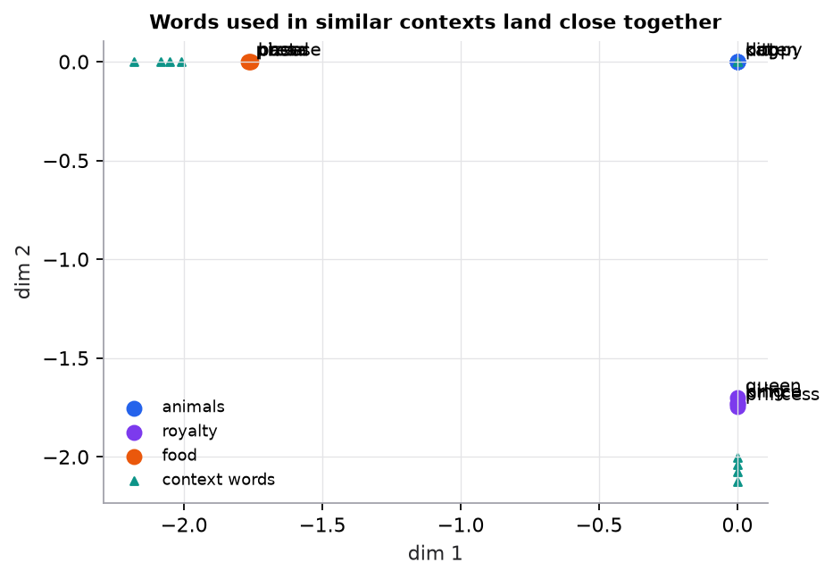
Synthetic corpus where each group of words appears with its own context words. A count-based method (co-occurrence, positive PMI, then SVD to 2 dimensions) recovers the three groups: cosine similarity is 0.997 for cat and dog but −0.997 for cat and king. Real embeddings are learned from billions of words and have hundreds of dimensions.
3. The math
Symbols
| Symbol | Meaning | Shape |
|---|---|---|
| vocabulary size | scalar | |
| embedding dimension | scalar | |
| embedding matrix (input vectors) | ||
| embedding of word (a row of ) | ||
| output ("context") vector of word | ||
| sigmoid |
Embedding lookup
A token ID selects row of . Equivalently, multiply a one-hot vector by : . Gradients during training update only the rows that were used.
Skip-gram with negative sampling
For each (center word , true context word ) pair, plus random "negative" words , maximize
That is binary classification: push the dot product up for real pairs and down for random pairs. Words that share contexts get pushed toward the same context vectors, so their embeddings become similar.
Count-based alternative
Build a word-word co-occurrence matrix, convert counts to positive pointwise mutual information, , and reduce dimensions with SVD. Word2Vec has been shown to implicitly factorize a matrix closely related to this one; the script uses this method because it needs no deep-learning library.
Worked example: similarity and analogy
Toy 3D embeddings: king , queen , man , woman .
Analogy. king − man + woman . Cosine with queen: dot ; norms and ; cosine . The nearest word to the analogy vector is "queen." (These numbers are hand-picked to illustrate the idea; real analogies hold only approximately.)
4. Implementation
Build it from scratch
We train skip-gram with negative sampling in about 50 lines of NumPy, on ten hand-written sentences about cats, dogs, mats, and rugs (synthetic, repeated 20 times). Two matrices are learned: input vectors and output vectors , both . is the embedding table you keep.
Training pairs from a window. Every word within 2 positions of a center word becomes a (center, context) pair. These pairs are the only labels; no human labelled anything.
def skipgram_pairs(docs, vocab, window=2):
    pairs = []
    for doc in docs:
        for i, center in enumerate(doc):
            for j in range(max(0, i - window), min(len(doc), i + window + 1)):
                if i != j:
                    pairs.append((vocab[center], vocab[doc[j]]))
    return np.array(pairs)
Predict: the sentence "the cat sat on the mat" has 6 words. How many pairs does it give with window 2? (Edge words have fewer neighbors.)
Where negatives come from. Negatives are drawn from word frequencies raised to the 3/4 power, as in the original Word2Vec. The power flattens the distribution so "the" is not drawn almost every time.
def noise_dist(docs, vocab):
    counts = np.zeros(len(vocab))
    for doc in docs:
        for t in doc:
            counts[vocab[t]] += 1
    p = counts ** 0.75                        # flattens: rare words sampled more than their frequency
    return p / p.sum()
Predict: one word appears 81 times and another once. With the 3/4 power, how many times more likely is the frequent word to be drawn? (81 is 3⁴.)
One gradient step. The loss for a pair is . Its derivative with respect to a score is for the true pair and for each negative. Each error multiplies the other side's vector to give that side's gradient.
def sgd_step(E, U, w, c, negs, lr):
    e = E[w].copy()                           # [d]
    g_pos = sigmoid(e @ U[c]) - 1.0           # d(loss)/d(score) for the true pair: pushes score up
    g_neg = sigmoid(U[negs] @ e)              # [k] for the negatives: pushes scores down
    E[w] -= lr * (g_pos * U[c] + g_neg @ U[negs])
    U[c] -= lr * g_pos * e
    np.subtract.at(U, negs, lr * g_neg[:, None] * e)   # safe if a negative repeats
    return -np.log(sigmoid(e @ U[c]) + 1e-9) - np.log(1 - g_neg + 1e-9).sum()
Predict: only rows w, c, and the negatives change. With , , , how many of the parameters can one step touch at most?
The loop. Shuffle the pairs each epoch and draw fresh negatives per pair.
def train(docs, vocab, d=16, window=2, k=5, epochs=60, lr=0.05, seed=42):
    rng = np.random.default_rng(seed)
    V = len(vocab)
    E = rng.normal(0, 0.1, (V, d))
    U = rng.normal(0, 0.1, (V, d))
    pairs, p = skipgram_pairs(docs, vocab, window), noise_dist(docs, vocab)
    for epoch in range(epochs):
        loss = 0.0
        for w, c in pairs[rng.permutation(len(pairs))]:
            loss += sgd_step(E, U, w, c, rng.choice(V, size=k, p=p), lr)
        if epoch in (0, epochs - 1):
            print(f"epoch {epoch + 1:3d}: mean loss per pair = {loss / len(pairs):.3f}")
    return E
Predict: "mat" and "rug" never appear in the same sentence. Will they end up close? Why?
Subwords for unseen words (the fastText idea). A static model has no vector for a word it never saw. fastText represents a word as the sum of vectors for its character n-grams (lengths 3 to 6, with < and > marking the word's start and end), so "kittenish" borrows from "kitten."
def char_ngrams(word, n_min=3, n_max=6):
    w = f"<{word}>"                           # boundary markers make prefixes and suffixes distinct
    return {w} | {w[i:i + n] for n in range(n_min, n_max + 1) for i in range(len(w) - n + 1)}
Predict: "
Use the library
In practice you train or load embeddings with a library (pip install gensim). sg=1 selects skip-gram, negative=5 sets , and gensim adds what our loop skips: subsampling of frequent words, a learning rate that decays, and multithreaded C code.
from gensim.models import Word2Vec, FastText
model = Word2Vec(sentences=tokenized_sentences, vector_size=100, window=5, sg=1, negative=5, min_count=5)
model.wv.most_similar("kitten")
ft = FastText(sentences=tokenized_sentences, vector_size=100, window=5, min_n=3, max_n=6)
ft.wv["kittenish"]          # works even if the word was never seen
In a neural network the embedding layer is the same table, trained with the rest of the model. A lookup is row indexing:
V, d = 10_000, 128
E = np.random.default_rng(0).normal(0, 0.1, (V, d))   # [V, d], learned during training
vectors = E[np.array([12, 845, 3])]                   # [3, d]
For most applications today, use a pretrained contextual encoder instead (pip install sentence-transformers):
from sentence_transformers import SentenceTransformer
encoder = SentenceTransformer("all-MiniLM-L6-v2")
vecs = encoder.encode(["my cat sleeps", "a kitten naps"], normalize_embeddings=True)
print(vecs[0] @ vecs[1])     # high similarity despite no shared words
Run it
From guide/ (takes a few seconds):
uv run code/09-classical-nlp/word2vec_scratch.pyKey output:
V = 24 words, 2800 training pairs per epoch
epoch   1: mean loss per pair = 2.590
epoch  60: mean loss per pair = 1.485
E shape: (24, 16)
nearest to cat : [('dog', 0.988), ('mouse', 0.831), ('mat', 0.569)]
nearest to mat : [('rug', 0.993), ('slept', 0.785), ('sat', 0.775)]
'kitten' has 19 n-grams; shares 14 with 'kittens', e.g. ['<ki', '<kit', '<kitt', '<kitte']
'kittenish' (never seen) still shares 14 n-grams with 'kitten'
"mat" and "rug" end up with cosine 0.993 without ever sharing a sentence, because both follow "on the." That is the distributional hypothesis, produced by 60 epochs of a binary classifier. The loss stays well above zero because the negatives are random and the corpus is tiny.
The figure script (count-based PPMI + SVD embeddings and the TF-IDF comparison) is code/09-classical-nlp/nlp.py.
5. Engineering
| Approach | Advantages | Limitations |
|---|---|---|
| TF-IDF + linear model | fast, cheap, interpretable, excellent baseline | sparse; no semantics beyond shared words |
| Static embeddings (Word2Vec, GloVe) | dense semantics, reusable | one vector per word; weak with ambiguity |
| Transformer embeddings | contextual, transferable | more compute, latency, and complexity |
Uses. Features for downstream models; semantic search and RAG (embed documents and queries, retrieve by cosine similarity); clustering and deduplication; recommendation (user and item embeddings).
Choosing an embedding model. Match the domain and language; check the maximum input length; benchmark on your retrieval or similarity task rather than trusting leaderboards; consider dimension (storage and speed) and whether vectors are normalized.
Bias. Embeddings learned from web text encode social biases present in that text (for example, gender associations with occupations). Audit before using them in decisions about people.
Watch outFailure modes. Out-of-vocabulary words with static embeddings (subword models fix this); ambiguous words averaged into one vector; mixing vectors from different embedding models in one index; re-embedding documents with a new model but not the queries (or vice versa).
Common mistakes
- Reading 2D projections of embeddings as exact geometry.
- Comparing unnormalized vectors with dot products when the model expects cosine.
- Assuming analogies always work; they are approximate and cherry-picked in demos.
6. Knowledge check
Quiz: Word embeddings
An embedding table has a vocabulary of 32,000 and dimension 512. How many parameters does it hold?
Practice exercise. An embedding matrix has a vocabulary of 50,000 tokens and dimension 768. How many parameters does it have, and what is the shape of the output for a batch of 8 sequences of 128 tokens?
Solution
parameters. Output shape .
Implementation challenge. Turn code/09-classical-nlp/word2vec_scratch.py into CBOW: average the input vectors of the context words within the window, and predict the center word with the same negative-sampling loss. Compare the nearest neighbors of "cat" and "mat" with skip-gram's.
Solution sketch
Build (context indices, center) examples instead of pairs. In the step, let h = E[ctx].mean(axis=0), score h @ U[center] and U[negs] @ h, and compute g_pos, g_neg exactly as before. The gradient for h is g_pos * U[center] + g_neg @ U[negs]; split it evenly over the context rows with np.subtract.at(E, ctx, lr * grad_h / len(ctx)). CBOW trains faster (one update per center word rather than per pair) and smooths over contexts, so neighbors of frequent words are similar to skip-gram's. Skip-gram usually does better for rare words, which get their own updates.
Summary
- Embeddings are dense vectors where words with similar contexts are close, learned by self-supervised prediction (skip-gram, CBOW) or count factorization.
- An embedding layer is a lookup table of shape .
- Cosine similarity compares embeddings; analogies are a fun but approximate property.
- Static embeddings give one vector per word; contextual (transformer) embeddings give one per occurrence.
Next: Named entity recognition
Related: From text to vectors · Self-attention · Model card: embedding model
Parts of this lesson are adapted from AI Engineering from Scratch by Rohit Ghumare (MIT license, notice): Word Embeddings — Word2Vec from Scratch, GloVe, FastText, and Subword Embeddings.
Interview angle
How does skip-gram with negative sampling learn word embeddings?
Slide a window over text to form (center word, context word) pairs. For each true pair , sample "negative" words from a smoothed unigram distribution (frequency raised to the 3/4 power). Then train a binary classifier: maximize , raising the dot product for real pairs and lowering it for random ones. Words that occur in similar contexts receive similar updates, pulled toward the same context vectors, so their embeddings end up close: the distributional hypothesis in action. Negative sampling replaces a softmax over the whole vocabulary, which costs per example, with binary classifications ( is typically 5 to 20), which makes training cheap. Only the embedding rows used in a batch get updated. Levy and Goldberg showed it implicitly factorizes a shifted PMI matrix.
Static embeddings or contextual transformer embeddings: when does each fit?
Static embeddings (Word2Vec, GloVe, fastText) give one vector per word type regardless of context, so "bank" in "river bank" and "bank account" share a single averaged vector. They're small, fast (a table lookup), and good features for lightweight models or tight compute budgets. Contextual embeddings from transformers compute a vector per token from the whole input, so ambiguity is resolved and word order matters; sentence-embedding models trained contrastively produce strong vectors for whole passages, the basis of semantic search and RAG. Costs: a forward pass per input, GPU or slower CPU inference, larger vectors, and versioning, since a new model means re-embedding the corpus. Rule of thumb: for retrieval, meaning-sensitive classification, or anything with ambiguity, use a modern embedding model benchmarked on your own data; use static embeddings when latency or footprint dominate, or as a baseline.
Semantic search quality collapsed right after you upgraded the embedding model. What happened?
Almost certainly an embedding-space mismatch: queries are embedded with the new model while the index still holds document vectors from the old one, or only partly re-embedded ones. Vectors from different models, even different versions of the same model, live in unrelated coordinate systems, so their cosine similarities are meaningless, even when the dimensions match. Check whether query and document vectors carry the same model version tag. Other suspects: the new model expects normalized vectors or cosine but the index uses raw inner product; it requires instruction prefixes such as "query: " and "passage: " for asymmetric search; its maximum input length is shorter, silently truncating chunks; or the dimension changed and the index was misconfigured. Fix: re-embed the entire corpus, store the model version with every vector, build the new index alongside the old one, and compare recall@k on a labeled query set before switching traffic.
You need to index 50 million documents with 1,024-dimensional float32 embeddings. How much memory do the vectors need, and how would you cut it?
bytes bytes, about 205 GB for the raw vectors, before index overhead (an HNSW graph adds more). Ways to cut it: store float16, halving it to about 102 GB with negligible quality loss; scalar-quantize to int8, about 51 GB, with a small recall loss that re-ranking recovers; product quantization to around 64 bytes per vector, about 3.2 GB, with a larger loss, so re-rank the top candidates using full vectors kept on disk; binary quantization at 128 bytes per vector as a fast first pass; or fewer dimensions, from a smaller model or one trained to allow truncation (Matryoshka embeddings), for example 256 dimensions. Measure recall@k against exact search on a labeled query set for each option, because the quality loss depends on the model and the data.