Module 9: Classical NLP 40 min10 min quick readNLP
Topic modeling
Discover the themes in an unlabeled corpus with LDA (documents as mixtures of topics, topics as distributions over words), implement collapsed Gibbs sampling, and choose between LDA, NMF, and embedding-based BERTopic.
Before this: From text to vectors, Word embeddings
Quick read: the intuition, interactive visualization, summary, and interview questions. The math, implementation, engineering, and knowledge-check sections are hidden.
Mental model. Imagine each document was written by someone who first rolled a weighted die to pick a theme for every word (60% finance, 40% AI), then picked a word from that theme's vocabulary list. Topic modeling runs this story backwards: from the words alone it recovers the vocabulary lists (topics) and each document's die weights (its topic mixture).
You will learn to
- State LDA's generative story and the two matrices it outputs: document-topic and topic-word .
- Compute one collapsed Gibbs sampling update by hand and implement the sampler.
- Explain why LDA takes raw counts, what and control, and how to choose the number of topics.
- Compare LDA, NMF, and BERTopic (embeddings plus clustering) and pick one for a given corpus.
- Evaluate topics with coherence, diversity, and human reading, and avoid treating a discovered topic as a real category.
Why it matters. You have 50,000 support tickets and no labels. Topic modeling gives a first map of what's in there: which themes exist, how big they are, and how they move over time. It feeds dashboards, triage, and labeling plans. It's also a standard interview topic because it tests probabilistic modeling, unsupervised evaluation, and judgment about when to stop trusting the output.
1. Intuition
Two outputs. A topic model returns:
- Topics: each is a probability distribution over the vocabulary. A finance topic puts high probability on "stocks", "rates", "inflation".
- Document mixtures: each document is a distribution over topics. A news story about chip stocks might be 60% finance and 40% AI.
That second point is mixed membership: a document can belong to several topics at once, unlike k-means, where every point belongs to exactly one cluster.
Word co-occurrence is the only signal. LDA never sees meaning. It notices that "stocks" and "yields" keep showing up in the same documents, so they probably come from the same topic. That's why it needs many documents, and why it struggles with very short ones: a 6-word tweet carries little co-occurrence evidence.
Learning by repeated guessing. Collapsed Gibbs sampling starts by giving every word token a random topic. Then, one token at a time, it removes that token's assignment and re-picks a topic with probability proportional to two things: how much this document already uses each topic, and how much each topic already uses this word. Repeat for every token, hundreds of times. Rich-get-richer dynamics pull related words into the same topic and keep each document focused on a few topics.
The embedding alternative. BERTopic skips the word-count story: it embeds each document with a sentence encoder, clusters the embeddings, and describes each cluster by its most distinctive words. It captures meaning (synonyms land together) but gives each document one main topic by default.
Key distinctionA discovered topic is a statistical pattern in word use, not a real category. "Topic 7" might be a genuine theme, a writing style, a boilerplate signature, or a language. Name topics only after reading documents from them.
2. Visualization
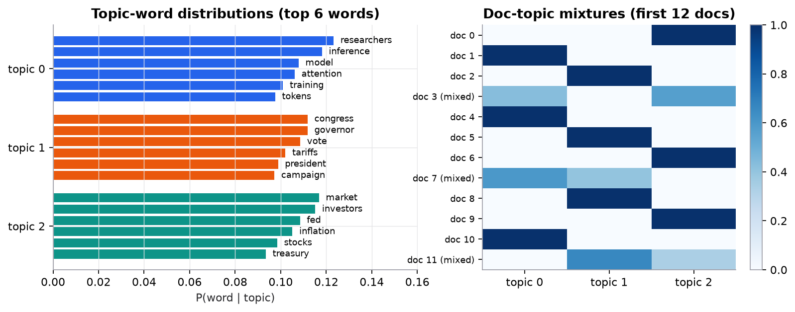
Synthetic corpus: 60 documents of 30 words drawn from three hand-written word lists of 10 words each. Every fourth document mixes two topics 60/40. LDA recovers the three lists exactly and assigns the mixed documents two-topic mixtures. Topic numbers are arbitrary: LDA does not know which list is "finance".
Try it (predict first, then run the script and check):
- Doc 3 was generated as 60% finance and 40% AI. Predict its inferred before looking at the output.
- Set
K=2in the firstgibbs_ldacall. Predict which two true topics get merged, and whether topic diversity drops. - Raise
alphafrom 0.1 to 5. Predict what happens to the heatmap's pure documents. - Feed sklearn's LDA a
TfidfVectorizermatrix instead of counts. Predict whether it errors, and whether the topics still make sense.
3. The math
Symbols
| Symbol | Meaning | Shape |
|---|---|---|
| number of documents, vocabulary size, number of topics | scalars | |
| topic mixture of document | , rows of | |
| word distribution of topic | , rows of | |
| topic assigned to the -th token of document | integer in | |
| Dirichlet prior on ; small means each document uses few topics | scalar (symmetric) | |
| Dirichlet prior on ; small means each topic uses few words | scalar (symmetric) | |
| tokens in document assigned to topic | ||
| times word is assigned to topic | ||
| total tokens assigned to topic |
The generative story
Only the words are observed. Inference recovers , , and . The model counts words, which is why LDA takes raw term counts (a bag of words), not TF-IDF weights.
Collapsed Gibbs update
"Collapsed" means and are integrated out, so we only sample the 's. For one token with word in document , with that token's own count removed (marked ):
After sampling, estimate
Worked example: one Gibbs update
topics, , , . The token is the word "model". With this token removed, its document has and tokens in each topic. Across the corpus "model" is assigned times to topic 0 and times to topic 1. Topic totals: , .
Denominators: and .
Normalize: the sum is , so and .
The document leans toward topic 0 (7 vs 2 tokens), but topic 0 has never produced "model", so the word factor wins. This is how LDA separates words: a topic that never uses a word almost never gets it.
Choosing K
There is no single right . Two cheap automatic signals:
- Topic diversity: the fraction of unique words across all topics' top- lists. 1.0 means no overlap; low values mean is too large and topics are splitting into near-duplicates.
- Topic coherence (, NPMI): do a topic's top words co-occur in a reference corpus more than chance? Higher is better.
In the script, diversity of the top 6 words is 1.00 for and , then 0.73 for and 0.58 for . Note that also scores 1.00 while merging two real topics: diversity catches too many topics, not too few. Read the topics.
4. Implementation
The full script is code/09-classical-nlp/topic_model_scratch.py (NumPy for the sampler, scikit-learn for the library comparison).
Build it from scratch
Step 1: map words to ids and start random. Every token gets a random topic. The three count tables are all the sampler needs: it never stores or while sampling.
def gibbs_lda(docs, K, alpha=0.1, beta=0.01, iters=200):
    vocab = sorted({w for d in docs for w in d})
    w2i = {w: i for i, w in enumerate(vocab)}
    V = len(vocab)
    W = [np.array([w2i[w] for w in d]) for d in docs]
    Z = [rng.integers(0, K, len(d)) for d in W]           # random initial topic per token
    ndk = np.zeros((len(W), K))                           # tokens in doc d assigned to topic k
    nkw = np.zeros((K, V))                                # times word w is assigned to topic k
    nk = np.zeros(K)                                      # tokens assigned to topic k
Predict: after initialization, roughly what fraction of a 30-token document's tokens is in each of 3 topics?
Step 2: fill the counts. One pass adds each token's random assignment to the three tables.
    for d, (ws, zs) in enumerate(zip(W, Z)):
        for w, z in zip(ws, zs):
            ndk[d, z] += 1
            nkw[z, w] += 1
            nk[z] += 1
Predict: what do ndk.sum(), nkw.sum(), and nk.sum() each equal?
Step 3: the sweep. For each token: subtract it from the counts (the in the formula), compute the unnormalized probabilities in one vectorized line, sample, and add it back under its new topic. Forgetting the subtraction counts the token as evidence for its own current topic.
    for _ in range(iters):
        for d, (ws, zs) in enumerate(zip(W, Z)):
            for i, (w, z) in enumerate(zip(ws, zs)):
                ndk[d, z] -= 1                            # remove this token's current assignment
                nkw[z, w] -= 1
                nk[z] -= 1
                p = (ndk[d] + alpha) * (nkw[:, w] + beta) / (nk + V * beta)   # [K]
                z = rng.choice(K, p=p / p.sum())          # resample its topic
                zs[i] = z
                ndk[d, z] += 1
                nkw[z, w] += 1
                nk[z] += 1
Predict: if beta were 0, what probability would a topic get for a word it has never been assigned?
Step 4: read off the estimates. Smoothed, normalized counts give and .
    theta = (ndk + alpha) / (ndk.sum(1, keepdims=True) + K * alpha)        # [D, K] doc-topic
    phi = (nkw + beta) / (nkw.sum(1, keepdims=True) + V * beta)            # [K, V] topic-word
    return theta, phi, vocab
Predict: with and , what is the smallest possible for a 30-token document?
Step 5: topic diversity.
def topic_diversity(tops):
    flat = [w for t in tops for w in t]
    return len(set(flat)) / len(flat)
Predict: 8 topics, 6 top words each, and 28 unique words among the 48. What is the diversity?
Use the library
scikit-learn's LDA uses online variational Bayes instead of Gibbs sampling; it is faster and deterministic for a fixed seed. Its priors are doc_topic_prior () and topic_word_prior (), both defaulting to . NMF factorizes the count (or TF-IDF) matrix with non-negative factors and is a fast, often sharper alternative.
from sklearn.feature_extraction.text import CountVectorizer
from sklearn.decomposition import LatentDirichletAllocation, NMF

cv = CountVectorizer(stop_words="english", min_df=2, max_df=0.9)   # raw counts; drop rare and ubiquitous words
X = cv.fit_transform(texts)                                          # [D, V] sparse
lda = LatentDirichletAllocation(n_components=10, random_state=0).fit(X)
doc_topic = lda.transform(X)                                         # [D, K], rows sum to 1
top = [cv.get_feature_names_out()[row.argsort()[::-1][:10]] for row in lda.components_]
nmf = NMF(n_components=10, init="nndsvd", random_state=0).fit(X)
For short or semantic text, BERTopic composes embeddings, dimensionality reduction, and clustering:
from bertopic import BERTopic   # pip install bertopic
topic_model = BERTopic(min_topic_size=15)                # default embeddings: all-MiniLM-L6-v2; UMAP; HDBSCAN
topics, probs = topic_model.fit_transform(texts)          # one topic id per doc; -1 = outliers
print(topic_model.get_topic_info().head())               # sizes and c-TF-IDF top words
Each cluster's words come from class-based TF-IDF: all documents in a cluster are concatenated into one, and a word scores , where is the average number of words per cluster and is the word's frequency over all clusters. min_topic_size defaults to 10. For mixtures, calculate_probabilities=True or approximate_distribution gives per-document topic distributions.
Run it
uv run code/09-classical-nlp/topic_model_scratch.pyKey lines of output:
unnormalised: topic0 = (7.1)(0.01)/150.3 = 0.000472, topic1 = (2.1)(9.01)/140.3 = 0.134861
normalised:   P(z=0) = 0.003, P(z=1) = 0.997

topic 0: researchers inference model attention training tokens
topic 1: congress governor vote tariffs president campaign
topic 2: market investors fed inflation stocks treasury
topic diversity (top 6): 1.00
doc 3: true mix [0.6 0.4 0. ], inferred theta [0.43 0.   0.56]
K = 5: diversity 0.73
K = 8: diversity 0.58
Doc 3 was 60% finance (topic 2 here) and 40% AI (topic 0), and LDA estimates 0.56 and 0.43. scikit-learn's LDA and NMF find the same three topics.
5. Engineering
When to pick what.
| Situation | Good default | Why |
|---|---|---|
| Long documents that mix themes (reports, articles) | LDA | mixed membership, cheap, works on any length |
| Short text (reviews, tweets, titles) | BERTopic or embeddings plus clustering | too few words for co-occurrence; embeddings carry meaning |
| CPU only, huge corpus, fast iteration | NMF or online LDA | sparse matrix math, minutes not hours |
| Need readable labels for stakeholders | any, then an LLM to name topics from top words and sample docs | names are for humans; check them |
Documents longer than the embedding model's context window must be chunked (and the chunk topics aggregated) for BERTopic; LDA has no length limit.
Preprocessing decides quality. Remove stop words and boilerplate (signatures, disclaimers, templates), or they become topics. Filter rare words (min_df) and near-universal ones (max_df). Lemmatize if inflections split topics. Bigrams help ("interest rate").
Evaluation. Combine automatic coherence (gensim CoherenceModel with coherence="c_v"), topic diversity, and a human read of the top words and 10 to 20 documents per topic. Perplexity on held-out text often disagrees with human judgments of quality, so don't choose by perplexity alone. Check stability: rerun with different seeds and see whether topics persist.
Production. Topic ids change between training runs, so freeze a model and map ids to names before building dashboards. To track trends, assign new documents with transform and watch topic shares over time. For BERTopic, watch the -1 outlier share; if it is large, lower min_topic_size or use reduce_outliers.
Common mistakes
- Feeding TF-IDF into LDA. LDA's likelihood is over counts; use
CountVectorizer. - Naming topics from top words alone, then reporting them as categories. Read documents first.
- Picking from one metric. Diversity misses merged topics; coherence can favor generic topics.
- Leaving boilerplate in, then finding a "topic" that is an email signature.
- Running LDA on 10-word documents and blaming the algorithm.
6. Knowledge check
Quiz: Topic modeling
How does LDA model a document?
Practice exercise. , , , . For a token of the word "vote", with the token removed: , ; , ; , . What is ?
Solution
Denominators are equal: . Topic 0: . Topic 1: . Sum . . The document is split evenly, so the word's history decides.
Implementation challenge. Add a perplexity estimate and a simple coherence score (average PMI of top-word pairs, computed from document co-occurrence in the same corpus) to the script. Plot both against and see whether they agree with topic diversity on the true .
Hint
PMI for words : , with probabilities as the fraction of documents containing the word or pair. Average it over all pairs of each topic's top 6 words, then over topics. Expect coherence to drop when topics split into near-duplicates that share words.
Summary
- LDA models documents as mixtures of topics and topics as distributions over words; it outputs and .
- Collapsed Gibbs sampling re-assigns each token with probability .
- Small gives focused documents, small gives focused topics; LDA needs raw counts.
- BERTopic (embeddings, UMAP, HDBSCAN, c-TF-IDF) wins on short semantic text; LDA wins on long mixed documents and low compute.
- Choose and judge quality with coherence, diversity, stability, and reading documents. Topics are patterns, not ground-truth categories.
Next: The neural-network forward pass
Related: Named entity recognition · From text to vectors · K-means · Density, hierarchical, and mixture clustering
Parts of this lesson are adapted from AI Engineering from Scratch by Rohit Ghumare (MIT license, notice): Topic Modeling — LDA and BERTopic.
Interview angle
Explain LDA's generative story and what you get out of it.
LDA assumes each topic is a probability distribution over the vocabulary, and each document has its own mixture over topics. To write a document, you repeatedly pick a topic from the document's mixture, then pick a word from that topic's distribution. Dirichlet priors control sparsity: a small alpha means each document uses few topics, and a small beta means each topic concentrates on few words. Only the words are observed, so inference runs the story backwards, usually with collapsed Gibbs sampling or variational Bayes. You get two matrices: document-topic theta, shape D by K, rows summing to 1, and topic-word phi, shape K by V. The key property is mixed membership: a document can be 60% finance and 40% AI, unlike k-means, which forces one cluster. It works on raw counts, so it needs bag-of-words input, not TF-IDF.
LDA or BERTopic for a corpus of 200,000 short product reviews? What about 5,000 long policy reports?
For short reviews, BERTopic or a similar embeddings-plus-clustering approach. Reviews have maybe 20 to 50 words, so word co-occurrence is sparse and LDA topics get noisy, while sentence embeddings put "battery dies fast" and "poor charge life" together even with no shared words. BERTopic embeds documents, reduces dimensions with UMAP, clusters with HDBSCAN, and names clusters with class-based TF-IDF. Watch the minus-one outlier bucket and set min_topic_size to the corpus scale. For long policy reports, LDA or NMF: each document genuinely mixes several themes, mixed membership is the point, and long documents would exceed an embedding model's context window unless chunked. LDA also runs cheaply on CPU. Either way I'd validate topics by reading documents, check stability across seeds, and have an LLM draft topic names that humans then confirm.
Your LDA run produces a topic whose top words are "regards", "thanks", "sent", "iphone", "please". What happened and how do you fix it?
LDA found a real co-occurrence pattern, just not a useful one: email signatures and boilerplate appear together in many documents, so they form their own topic. It's a preprocessing failure, not an algorithm failure. Fixes: strip signatures, quoted replies, and templates before vectorizing; add domain stop words; set max_df around 0.5 to 0.9 to drop words that appear in most documents; and set min_df to drop typos and one-off tokens. Then rerun and compare coherence and diversity, and read 10 to 20 documents per topic. More generally, junk topics come from boilerplate, different languages, or formatting artifacts. Treat every topic as a hypothesis about the corpus that you confirm by reading documents, not as a category, and freeze the preprocessing with the model so production assignments stay consistent.
Do one collapsed Gibbs update: alpha 0.1, beta 0.01, V 30. The document has 7 tokens in topic 0 and 2 in topic 1; the word has 0 assignments to topic 0 and 9 to topic 1; topic totals are 150 and 140.
The update is proportional to (n_dk plus alpha) times (n_kw plus beta) divided by (n_k plus V times beta), with the current token removed from all counts. V times beta is 30 times 0.01, or 0.3. Topic 0: 7.1 times 0.01 divided by 150.3, which is 0.000472. Topic 1: 2.1 times 9.01 divided by 140.3, which is 18.921 over 140.3, or 0.1349. The sum is about 0.1353, so the token goes to topic 1 with probability 0.997 and topic 0 with 0.003. The document prefers topic 0, but topic 0 has never used this word, and beta is tiny, so the word factor dominates. That's the mechanism that separates vocabularies across topics. A larger beta would soften it, letting topics share words more.