Module 14: Transformers 35 min9 min quick readTransformers
BERT and masked language modeling
Pretrain an encoder by hiding tokens and predicting them from both sides, implement the 80/10/10 masking rule and the loss mask, and decide when an encoder beats a decoder.
Before this: Self-attention, The transformer architecture
Quick read: the intuition, interactive visualization, summary, and interview questions. The math, implementation, engineering, and knowledge-check sections are hidden.
Mental model. GPT reads a sentence left to right and guesses the next word. BERT does a cloze test: some words are blanked out, and it fills each blank using the words on both sides. A model trained that way can't write text, but it builds very good representations of text it has already been given.
You will learn to
- Explain masked language modeling (MLM) and why it needs a bidirectional encoder.
- Implement the 80/10/10 masking rule and the
-100loss mask. - Compute the MLM loss on the masked positions and compare its training signal per token with next-token prediction.
- Describe what RoBERTa, ELECTRA, and ModernBERT changed.
- Choose between an encoder and a decoder for classification, retrieval, reranking, and generation.
Why it matters. Most search, retrieval, classification, and reranking systems still run on encoders: embedding models and cross-encoder rerankers are fine-tuned BERT-style models. They are small, fast (one forward pass, no generation loop), and accurate on understanding tasks. "Encoder versus decoder" and "how is BERT trained" are standard interview questions.
1. Intuition
A decoder like GPT uses a causal mask: token only sees tokens before it. That is required for generation, because the future doesn't exist yet when you are writing. But when the whole input is already known (a review to classify, a document to embed), throwing away the right-hand context wastes information.
BERT (Devlin et al., 2018) is the transformer encoder with no attention mask: every token attends to every token. Training it with "predict the next word" would be trivial, since each position can see the answer. So BERT hides the answer instead:
- Pick about 15% of token positions.
- Replace most of them with a special
[MASK]token. - Ask the model to predict the original token at those positions, using context from both sides.
Take "the cat sat on the mat." Blank out sat. Reading left to right you have only "the cat ___": it could be sat, ran, slept. Reading both sides, "the cat ___ on the mat", makes sat far more likely. The script makes this concrete on synthetic sentences: guessing a blank verb from the left neighbour alone gets 33% right; using both neighbours gets 100%.
Two details matter in practice:
- The 80/10/10 rule.
[MASK]never appears when you later fine-tune or use the model. If the model only learned to predict at[MASK]positions, it might not build good representations of real tokens. So of the chosen positions, 80% become[MASK], 10% become a random token, and 10% stay unchanged. The model can't tell which visible tokens are corrupted, so it must represent every token well. - Special tokens.
[CLS]is prepended; its final vector is used as a sentence summary for classification.[SEP]separates two segments, such as a query and a document.
After pretraining, you add a small head (a linear layer on [CLS] for classification, or on every token for tagging) and fine-tune.
2. Visualization
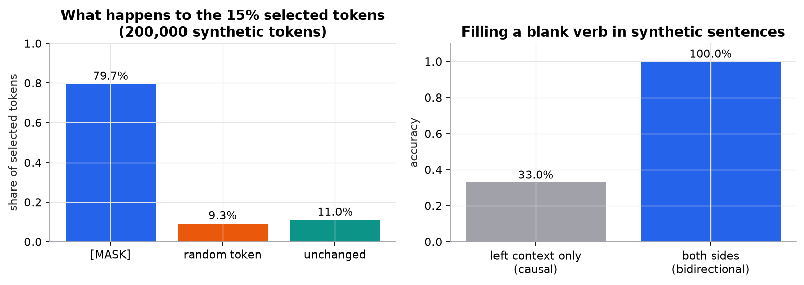
Synthetic data. Left: the 80/10/10 rule measured on 200,000 random token ids. "Unchanged" is a little above 10% because a random replacement sometimes draws the original token. Right: a count-based predictor (no neural network) fills a blank verb in a tiny synthetic grammar where the word after the verb ("on", "in", "home") identifies it.
Try it (edit the script, predict first, then run):
- In
mask_tokens, changep=0.15top=0.5. Predict the "selected" percentage and whether the 80/10/10 split changes. - Delete the
can &guard so special tokens can be masked. What would the model learn to predict at[CLS], and why is that wasted capacity? - In the synthetic grammar, make "sat" and "ran" both followed by "on". Predict the both-sides accuracy before running.
- Change the blank from the verb (position 2) to the subject (position 1). Does seeing the right side help now? Why not?
3. The math
Symbols
| Symbol | Meaning | Shape |
|---|---|---|
| original token ids | ||
| corrupted input after masking | ||
| set of positions chosen for prediction | subset of | |
| selection rate (0.15 in BERT) | scalar | |
| encoder output, one vector per token | ||
| output projection to the vocabulary | ||
| vocabulary size (30,522 for BERT's WordPiece) | scalar |
The objective
The encoder reads the corrupted sequence with no attention mask. For each chosen position , a softmax over the vocabulary predicts the original token:
Positions outside contribute nothing. In code they get the label -100, which PyTorch's cross-entropy ignores by default.
Compare the decoder objective, which predicts every position from its left context: .
Worked example: the loss on one sentence
Sentence: [CLS] the cat sat on the mat [SEP], 8 tokens, 6 of them maskable. Suppose positions cat and mat are chosen. cat is replaced by [MASK] (the 80% case); mat is left unchanged (the 10% case), so the model sees mat but is still asked to predict it.
The model gives the correct token probability 0.5 at cat and 0.2 at mat:
The other six positions have label -100 and add nothing.
Worked example: training signal per sequence
A 512-token sequence (BERT's maximum) with 2 special tokens has 510 maskable tokens:
- MLM predicts about tokens per sequence.
- A decoder predicts all 511 next tokens of a 512-token sequence.
- So MLM gets of a decoder's prediction targets for the same forward pass.
That inefficiency motivated ELECTRA (Clark et al., 2020): a small generator fills the blanks, and the main model classifies every token as original or replaced, so all positions give a training signal.
Model size
BERT-base has 12 layers, , 12 heads, and about 110M parameters; BERT-large has 24 layers, , 16 heads, and about 340M. The transformer architecture lesson's parameter count applies unchanged; only the mask and the objective differ from GPT.
4. Implementation
Build it from scratch
The full script is code/14-transformers/bert_mlm.py (NumPy only). It builds the masking, then shows why bidirectional context helps. The encoder itself is the transformer block with no causal mask, so the new code is all in the data.
First choose positions and build labels. Labels hold the original id at chosen positions and -100 everywhere else, so the loss only sees the blanks.
def mask_tokens(ids, rng, p=0.15):
    ids = np.array(ids)
    labels = np.full_like(ids, IGNORE)
    can = ~np.isin(ids, list(SPECIAL))             # never mask [CLS], [SEP], [PAD]
    chosen = can & (rng.random(len(ids)) < p)      # pick ~15% of positions
    labels[chosen] = ids[chosen]                   # loss only on chosen positions
Predict: labels are set from ids before any corruption. What would go wrong if you set them after replacing tokens with [MASK]?
Then corrupt the chosen positions. One random draw per position decides which of the three cases it falls in.
    r = rng.random(len(ids))
    inputs = ids.copy()
    inputs[chosen & (r < 0.8)] = ID["[MASK]"]      # 80%: [MASK]
    rand = chosen & (r >= 0.8) & (r < 0.9)         # 10%: a random real token
    inputs[rand] = rng.integers(len(SPECIAL), len(VOCAB), rand.sum())
    return inputs, labels                          # remaining 10%: unchanged
Predict: with 16 real tokens in the vocabulary, how often does the "random token" case pick the original token by accident? (1 in 16, so about 0.6% of selected tokens move from "random" to "unchanged": the script measures 9.3% and 11.0%.)
Tokenizers split rare words into pieces such as un ##believ ##able. Masking one piece leaves the others as a giveaway. Whole-word masking groups the pieces and masks a whole word at once:
def whole_word_spans(pieces):
    """Group WordPiece-style tokens: a piece starting with '##' continues the previous word."""
    spans, start = [], 0
    for k in range(1, len(pieces) + 1):
        if k == len(pieces) or not pieces[k].startswith("##"):
            spans.append((start, k))
            start = k
    return spans
Predict: if only ##believ were masked, how hard is it to guess from un [MASK] ##able? That is why whole-word masking makes the task harder and the representations better.
Finally, why both sides help. The script trains two count-based predictors on synthetic sentences: one sees the left neighbour (like a decoder), one sees left and right (like an encoder), and both fill a blank verb.
for s in train:
    for k in range(1, len(s)):
        left[(s[k - 1], s[k])] += 1                       # left neighbour only (GPT-style)
        right = s[k + 1] if k + 1 < len(s) else "</s>"
        both[(s[k - 1], right, s[k])] += 1                 # left AND right (BERT-style)
Predict: the left neighbour of every verb is "cat" or "dog", and there are three verbs. Roughly what accuracy can the left-only predictor reach?
Use the library
Hugging Face implements exactly this rule in its data collator; the encoder and MLM head come pretrained:
from transformers import AutoTokenizer, AutoModelForMaskedLM, DataCollatorForLanguageModeling, pipeline

tok = AutoTokenizer.from_pretrained("bert-base-uncased")
collator = DataCollatorForLanguageModeling(tok, mlm_probability=0.15)   # 80/10/10 and -100 labels
batch = collator([tok("the cat sat on the mat")])
print(batch["input_ids"], batch["labels"])

fill = pipeline("fill-mask", model="bert-base-uncased")
print(fill("the cat [MASK] on the mat.")[:3])          # top guesses, using both sides
What the library adds: subword tokenization with [CLS]/[SEP] inserted, dynamic masking (a new random mask every time a batch is built, which RoBERTa showed helps), padding with attention masks, and a tied output layer. For new projects, ModernBERT (answerdotai/ModernBERT-base, Warner et al., 2024) is a drop-in modern encoder: RoPE positions, GeGLU feed-forward layers, alternating local and global attention (the attention variants lesson), and an 8,192-token context instead of 512. Embedding models (sentence-transformers) and cross-encoder rerankers are BERT-style encoders fine-tuned with different losses.
Run it
From guide/:
uv run code/14-transformers/bert_mlm.pyselected 15.02% of tokens; of those: [MASK] 79.69%, random 9.26%, unchanged 11.05%
(a random draw can pick the original token, so 'unchanged' sits slightly above 10%)
whole-word spans: ['the', 'un ##believ ##able', 'cat', 'play ##ed']
fill the verb blank on 500 synthetic test sentences:
left context only : 33.0%
both sides : 100.0%The expected split is 80%, , and ; the measured values differ by sampling noise on about 30,000 selected tokens. The left-only predictor always guesses the most common verb after "cat" or "dog", about one in three; the word after the verb gives it away to the both-sides predictor.
5. Engineering
When to pick an encoder.
| Task | Encoder (BERT-style) | Decoder (GPT-style) |
|---|---|---|
| Classification (intent, sentiment, toxicity) | one forward pass, small, cheap to fine-tune | works zero-shot, costs more per request |
| Token tagging (NER, PII detection) | native: one output per token, sees both sides | awkward: must generate labels |
| Embeddings for retrieval | standard (bi-encoders) | possible with LLM-based embedders, larger |
| Reranking for RAG | standard (cross-encoders read query and document together) | LLM rerankers, slower |
| Generating text | not suitable | the right tool |
What changed since 2018. RoBERTa (Liu et al., 2019) dropped BERT's second objective, next-sentence prediction, trained longer on more data with dynamic masking, and improved results. ELECTRA made every token a training target. ModernBERT updated the block with the same pieces modern decoders use and extended the context to 8,192 tokens.
Compute and serving. A 110M-parameter encoder classifies a 128-token input in one forward pass on a CPU, with no KV cache or decoding loop. Throughput is limited by batch size and sequence length; truncate or chunk long inputs, since original BERT stops at 512 tokens.
Fine-tuning. Fine-tune the whole encoder with a small learning rate (around 2e-5 to 5e-5) for a few epochs, or freeze it and train a head when labels are scarce. Encoders overfit small datasets quickly; keep a validation set and stop early.
Watch outFailure modes. Using
[CLS]from a model that was never fine-tuned as a sentence embedding (raw BERT's[CLS]vectors are poor for similarity; use a model trained for embeddings); inputs silently truncated at 512 tokens; a tokenizer that doesn't match the checkpoint; trying to generate text with an encoder.
Common mistakes
- Computing the loss over all positions instead of only masked ones (forgetting the
-100labels). - Masking special or padding tokens.
- Always replacing with
[MASK](no 10/10), which creates a mismatch between pretraining and fine-tuning inputs. - Reaching for a large decoder for high-volume classification where a fine-tuned encoder is cheaper and often as accurate.
- Comparing an encoder's MLM loss with a decoder's next-token loss: they are different tasks, so the numbers are not comparable.
6. Knowledge check
Quiz: BERT and masked language modeling
What is BERT's main pretraining objective?
Practice exercise. A batch has 32 sequences of 128 tokens, each with [CLS] and [SEP]. With and the 80/10/10 rule, about how many positions get a label, and how many of those inputs are [MASK], random, and unchanged?
Solution
Maskable tokens: . Labelled: , about 605. Of those, [MASK]: ; random: ; unchanged: . All 605 contribute to the loss, including the ones the model can see unchanged. The remaining positions (including the 64 special tokens) have label -100.
Implementation challenge. Add a whole_word_mask(pieces, rng, p) function that uses whole_word_spans, selects each word with probability , and applies the 80/10/10 choice once per word to all its pieces. Check on 10,000 synthetic sentences that the fraction of selected words is close to .
Solution
def whole_word_mask(pieces, rng, p=0.15):
    inputs, labels = list(pieces), [None] * len(pieces)
    for a, b in whole_word_spans(pieces):
        if rng.random() >= p:
            continue
        r = rng.random()                      # one decision for the whole word
        for k in range(a, b):
            labels[k] = pieces[k]
            if r < 0.8:
                inputs[k] = "[MASK]"
            elif r < 0.9:
                inputs[k] = rng.choice(VOCAB[len(SPECIAL):])
    return inputs, labels
Count selected words, not pieces: a word counts once even if it has three pieces. The fraction converges to ; the fraction of selected pieces is higher than when long words are common, because each selected long word labels several pieces.
Summary
- BERT is a transformer encoder with no attention mask, pretrained by predicting hidden tokens from both sides.
- About 15% of tokens are selected; 80% become
[MASK], 10% random, 10% unchanged, and only selected positions enter the loss. - MLM gets a training signal from roughly 15% of positions, against 100% for next-token prediction, which motivated ELECTRA.
- Encoders remain the default for classification, tagging, embeddings, and reranking; decoders are for generation.
- RoBERTa dropped next-sentence prediction; ModernBERT brought RoPE, GeGLU, local/global attention, and 8k context.
Next: Attention variants
Related: The transformer architecture · Word embeddings · Tokenization and pretraining · The RAG pipeline
Go deeper, code-first (AI Engineering from Scratch): T5, BART — Encoder-Decoder Models
Parts of this lesson are adapted from AI Engineering from Scratch by Rohit Ghumare (MIT license, notice): BERT — Masked Language Modeling.
Interview angle
How is BERT pretrained, and why can't it just predict the next token?
BERT is a transformer encoder with no causal mask, so every position attends to every other. If you trained it to predict the next token, each position could simply read the answer from the input. Instead it uses masked language modeling: select about 15% of tokens, corrupt them, and predict the originals at those positions from context on both sides. The loss is cross-entropy over the vocabulary, averaged only over selected positions; the rest get label minus 100 and are ignored. Of the selected tokens, 80% become the MASK token, 10% become a random token, and 10% stay unchanged. That mix exists because MASK never appears at fine-tuning time, and because the model can't tell which visible tokens are corrupted, it has to build good representations of every token. Original BERT also had next-sentence prediction, which RoBERTa showed was unnecessary.
For a high-volume intent classifier, would you fine-tune a BERT-style encoder or prompt an LLM?
With a few thousand labelled examples, I'd start by fine-tuning a small encoder. It reads the whole input bidirectionally, gives the answer in one forward pass, and a 100M to 400M parameter model runs cheaply on CPUs or small GPUs at very high throughput with tight latency. Fine-tuning takes minutes, and accuracy on a fixed label set is usually competitive with much larger models. An LLM wins when there are no labels, when classes change often, or when the output needs explanation or open-ended text. A common path is to prompt an LLM to label data, check a sample by hand, then train the encoder on those labels and serve it. I'd decide on measured accuracy, latency at p95, and cost per million requests on a held-out set, not on model size.
You took raw BERT's CLS vector as a sentence embedding for semantic search and results are poor. Why?
Raw BERT was never trained to make CLS vectors of similar sentences close. Its pretraining objective is token prediction, so CLS carries whatever helped that objective and wasn't tuned for cosine similarity. The space is also anisotropic: vectors cluster in a narrow cone, so most pairs look similar. Mean pooling helps a little but doesn't fix the core problem. The fix is a model trained for embeddings: a sentence-transformers style bi-encoder fine-tuned with a contrastive loss on query and passage pairs, or a current embedding model. Then evaluate on your own labelled queries with recall at k. For the final ordering, add a cross-encoder reranker, which reads the query and document together in one bidirectional pass and is more accurate on the top candidates.
Per 512-token sequence, how many prediction targets does MLM give versus a GPT-style model, and what follows?
With two special tokens, 510 tokens are maskable, and 15% of 510 is about 76.5 targets. A decoder predicts every next token: 511 targets in a 512-token sequence. So MLM gets roughly 15% of the training signal from the same forward and backward pass. Two things follow. First, encoders need more compute per useful prediction, which is why ELECTRA replaced MLM with replaced-token detection: a small generator fills the blanks and the main model classifies every token as original or replaced, so all 510 positions train it. Second, raising the mask rate isn't free: with too many tokens hidden, there is too little context left to predict from. Some later work found rates above 15% can still help larger models, so the rate is a tunable hyperparameter, not a law.