Module 27: Training at scale 40 min10 min quick readDeep learning
Collective operations from scratch
Build ring reduce-scatter, all-gather, and all-reduce, prove the 2(N-1)/N bandwidth cost, and pick ring or tree with a latency-bandwidth model.
Before this: Gradient descent, Vectors and matrices
Quick read: the intuition, interactive visualization, summary, and interview questions. The math, implementation, engineering, and knowledge-check sections are hidden.
Mental model. Four GPUs each hold a different set of numbers and all need the total. Shouting everything to one leader overloads the leader. Passing pieces around a circle, each person adding their part and handing it on, keeps every link equally busy and finishes in the same time however many people join.
You will learn to
- Define all-reduce, reduce-scatter, all-gather, and broadcast by what each rank holds before and after.
- Implement ring reduce-scatter and all-gather, and compose them into ring all-reduce.
- Derive that a ring all-reduce sends times the tensor per rank, and compare it with a parameter server.
- Use a latency-bandwidth (-) cost model to explain when tree algorithms beat rings, and why frameworks bucket gradients.
Why it matters. Every multi-GPU training method in this module is built from these four operations. Data parallelism is one all-reduce per step; ZeRO is a reduce-scatter plus an all-gather; FSDP all-gathers weights before each layer. If you know what each one costs, you can predict a training job's communication time on paper and explain why it scales or stalls.
1. Intuition
Picture GPUs (called ranks), each holding a tensor of the same shape: for example its own gradients after a backward pass on its own data.
| Operation | Before | After |
|---|---|---|
| All-reduce | each rank has its own tensor | every rank has the sum (or mean) of all of them |
| Reduce-scatter | each rank has its own tensor, split into chunks | each rank has the sum of one chunk |
| All-gather | each rank has one chunk | every rank has all chunks, concatenated |
| Broadcast | one rank has a tensor | every rank has a copy |
The key identity: all-reduce = reduce-scatter + all-gather. First each rank becomes responsible for summing one slice; then everyone shares their finished slice.
Parameter server. The obvious design sends every tensor to one rank, sums, and sends the result back. The server's link carries tensors in and out, so the time grows with .
Ring. Arrange ranks in a circle. Split each tensor into chunks. In each step every rank sends one chunk to its right neighbour and receives one from its left, adding it to its own copy of that chunk. After steps each rank has the complete sum of one chunk (reduce-scatter). Another steps pass the finished chunks around (all-gather). Every link is busy every step and no rank is special.
Tree. For a broadcast, the rank with the data sends to one other, then both send to two more, then four send to four more. ranks are reached in rounds. Trees take fewer steps, which matters when each message has a fixed startup cost.
2. Visualization
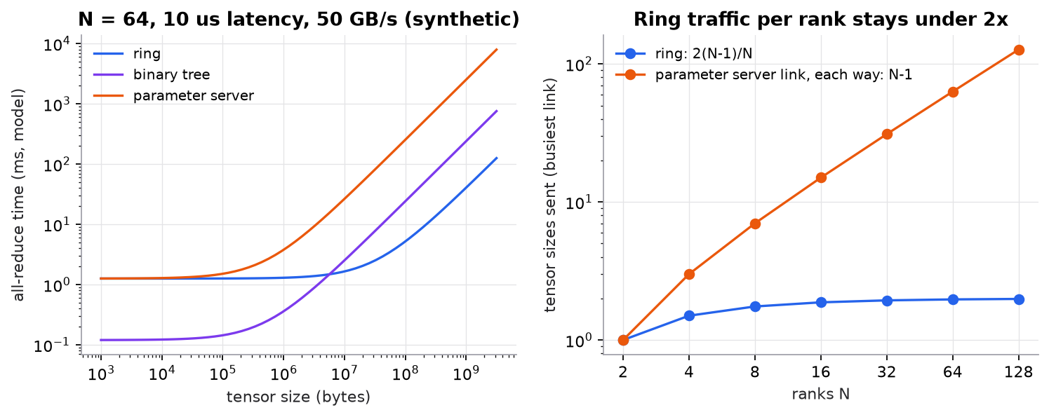
A model, not a measurement: synthetic link with 10 microseconds per message and 50 GB/s. Real libraries such as NCCL use pipelined and hierarchical variants whose crossover points depend on the hardware.
Try it (predict first, then run code/27-training-at-scale/collectives.py and edit it):
- Set
N, T = 8, 16. Predict the number of ring steps and the floats sent per rank before running. - Change
alphato100e-6(a slow network). Predict whether the ring-tree crossover moves to bigger or smaller tensors. - In
reduce_scatter, predict which chunk index rank 2 ends up holding with . Check the printout. - Change
tree_broadcast(8, ...)to 9 ranks. Predict the number of rounds and sends.
3. The math
Symbols
| Symbol | Meaning | Unit |
|---|---|---|
| number of ranks (GPUs) | count | |
| tensor size | bytes | |
| startup latency per message | seconds | |
| time per byte on one link (1 / bandwidth) | seconds per byte |
Ring all-reduce
Each chunk has bytes. Reduce-scatter takes steps, each rank sending one chunk per step; all-gather takes another .
As grows the bandwidth term tends to : it does not grow with the number of ranks. The latency term grows linearly with .
Reduce-scatter and all-gather alone each cost half: .
Parameter server and binary tree
The server's single link carries full tensors each way. A simple binary tree reduces up and broadcasts down in rounds, each moving the whole tensor. Trees win when dominates (small messages), rings when dominates (large messages). Production libraries use pipelined trees and hierarchical schemes that do better than this naive tree; NCCL picks an algorithm per call based on message size and topology.
Worked example: four ranks, eight numbers each
Ranks hold (synthetic integers):
| Rank | Tensor |
|---|---|
| 0 | [8, 6, 5, 2, 3, 0, 0, 0] |
| 1 | [1, 8, 6, 9, 5, 6, 9, 7] |
| 2 | [6, 5, 5, 9, 2, 8, 6, 0] |
| 3 | [3, 8, 5, 0, 7, 7, 8, 1] |
Split into chunks of 2. The column sums are [18, 27 | 21, 20 | 17, 21 | 23, 8].
- Step . Rank sends its chunk to rank , which adds it to its own copy. Rank 1 receives rank 0's chunk 0, [8, 6], and adds it to its own [1, 8]: [9, 14].
- Step . Rank sends chunk (the partial sum it just updated). Rank 2 receives rank 1's chunk 0, [9, 14], and adds its own [6, 5]: [15, 19].
- Step . Rank 3 receives chunk 0, [15, 19], and adds [3, 8]: [18, 27]. That is the full sum of chunk 0.
- After reduce-scatter: rank 3 holds chunk 0 = [18, 27]; rank 0 holds chunk 1 = [21, 20]; rank 1 holds chunk 2 = [17, 21]; rank 2 holds chunk 3 = [23, 8]. With this schedule rank finishes chunk ; libraries relabel the chunks so rank owns chunk .
- All-gather: 3 more steps pass the finished chunks around. Every rank ends with [18, 27, 21, 20, 17, 21, 23, 8].
- Traffic: steps, each sending one 2-float chunk, so floats per rank . ✓
Worked example: gradients of a 7B-style model
A 7B-style model has parameters. Its bf16 gradients are bytes GB. Ring all-reduce over sends GB per GPU per step. At 50 GB/s per link (synthetic) that is s of pure transfer, unless it overlaps with the backward pass.
4. Implementation
Build it from scratch
We simulate ranks in one process. A Ring moves one array per rank to its right neighbour per step and counts what each rank sends, so we can check the formula.
class Ring:
    """N ranks on a ring. A step is synchronous: every rank sends one chunk to its right neighbour."""

    def __init__(self, n):
        self.n = n
        self.sent = [0] * n      # floats sent by each rank
        self.steps = 0

    def shift(self, outgoing):
        """outgoing[r] is what rank r sends to rank r+1. Returns what each rank receives."""
        for r, x in enumerate(outgoing):
            self.sent[r] += x.size
        self.steps += 1
        return [outgoing[(r - 1) % self.n] for r in range(self.n)]
Predict: in one shift, how many arrays cross the network in total?
Reduce-scatter: at step s rank r sends chunk (r - s) mod N and adds what it receives into chunk (r - s - 1) mod N. The chunk it sends is always the one it updated in the previous step, so partial sums travel around the ring and grow.
def reduce_scatter(ring, tensors):
    """Ring reduce-scatter. After N-1 steps rank r holds the full sum of chunk (r + 1) mod N."""
    n = ring.n
    chunks = [np.array_split(t.astype(np.float64), n) for t in tensors]   # chunks[rank][chunk]
    for s in range(n - 1):
        send_idx = [(r - s) % n for r in range(n)]
        received = ring.shift([chunks[r][send_idx[r]] for r in range(n)])
        for r in range(n):
            idx = (r - s - 1) % n                       # the chunk my left neighbour just sent
            chunks[r][idx] = chunks[r][idx] + received[r]
    return [((r + 1) % n, chunks[r][(r + 1) % n]) for r in range(n)]    # (chunk index, summed chunk)
Predict: if one rank's tensor contained a NaN in chunk 2, which ranks would end up with a NaN after reduce-scatter? After all-gather?
All-gather passes each finished chunk to the right times. All-reduce is the two composed.
def all_gather(ring, owned, n_chunks):
    """Ring all-gather. owned[r] = (chunk index, data). After N-1 steps every rank has every chunk."""
    n = ring.n
    have = [{i: d} for i, d in owned]
    carry = list(owned)
    for _ in range(n - 1):
        ring.shift([d for _, d in carry])               # count the sends
        carry = [carry[(r - 1) % n] for r in range(n)]  # pass (index, data) to the right
        for r in range(n):
            have[r][carry[r][0]] = carry[r][1]
    return [np.concatenate([h[i] for i in range(n_chunks)]) for h in have]

def all_reduce(ring, tensors):
    """Ring all-reduce = reduce-scatter, then all-gather of the summed chunks."""
    return all_gather(ring, reduce_scatter(ring, tensors), ring.n)
Predict: all-gather does no arithmetic. Why does it still cost as many bytes as reduce-scatter?
The cost models are one line each:
def t_ring(n, T, alpha, beta):
    return 2 * (n - 1) * alpha + 2 * (n - 1) / n * T * beta

def t_tree(n, T, alpha, beta):
    """Reduce up a binary tree, then broadcast down: 2 log2(N) rounds, each moving the full tensor."""
    return 2 * np.log2(n) * (alpha + T * beta)
Predict: at , for which tensor size do the two times match? (Set them equal and solve for .)
Use the library
On GPUs, torch.distributed with the NCCL backend runs these as optimized kernels over NVLink and InfiniBand:
import torch.distributed as dist
dist.init_process_group("nccl")                 # launched with torchrun --nproc-per-node=8
dist.all_reduce(grad, op=dist.ReduceOp.SUM)     # in place on every rank
dist.reduce_scatter_tensor(shard_out, full_in)  # shard_out has numel / world_size
dist.all_gather_into_tensor(full_out, shard_in)
dist.broadcast(weights, src=0)
You rarely call these directly. DistributedDataParallel groups gradients into buckets (bucket_cap_mb, 25 MB by default) and launches one all-reduce per bucket as soon as backward has filled it, so communication overlaps with the rest of backward. FSDP and DeepSpeed ZeRO issue the reduce-scatters and all-gathers for you.
Run it
uv run code/27-training-at-scale/collectives.pyKey lines:
  after reduce-scatter rank 0 holds chunk 1 = [21, 20]
  after reduce-scatter rank 3 holds chunk 0 = [18, 27]
  after all-gather every rank equals the sum: True
  steps = 6 (= 2(N-1)); floats sent per rank = [12, 12, 12, 12] (2(N-1)/N x T = 12)
  N = 1024: 2(N-1)/N = 1.9980 GB
3) Tree broadcast to 8 ranks: 3 rounds (log2 8), 7 sends, all have it: True
     0.004 MB: ring     1.260 ms  tree     0.121 ms  server     1.270 ms
  1000.000 MB: ring    40.635 ms  tree   240.120 ms  server  2521.260 ms
5. Engineering
Bucket small tensors. A model has hundreds of parameter tensors. One all-reduce each would pay the latency hundreds of times. Bucketing turns them into a few large messages, where the ring's bandwidth term dominates.
Overlap with backward. Gradients of the last layers are ready first. DDP starts their all-reduce while earlier layers are still computing, hiding much of the communication. If communication still exceeds compute, the GPUs wait: check a profiler for idle gaps.
Topology matters. Inside a node, GPUs talk over NVLink at hundreds of GB/s; between nodes, over InfiniBand or Ethernet at roughly an order of magnitude less per GPU. Libraries run hierarchical collectives: reduce inside the node first, then across nodes. This is why tensor parallelism stays inside a node and data parallelism spans nodes.
Straggler effect. A ring is synchronous: every step waits for the slowest link. One slow GPU, a degraded cable, or a noisy neighbour slows every rank. Collective timeouts (NCCL_TIMEOUT, timeout= in init_process_group) turn a hang into an error you can debug.
Precision of the sum. Summing many bf16 gradients loses precision. Frameworks often reduce in fp32, or average rather than sum, to stay in range.
Common mistakes
- Thinking all-reduce traffic grows with : per rank it approaches and stops.
- Forgetting to divide by after a SUM all-reduce in data parallelism, which multiplies the effective learning rate by .
- Calling collectives in different orders on different ranks (for example inside an
if rank == 0block): every rank waits forever. Every rank must make the same collective calls in the same order. - Measuring communication cost with tiny tensors and extrapolating: small messages are latency-bound and give the wrong picture.
- Ignoring the latency term at large : grows with ranks, which is one reason hierarchical and tree algorithms exist.
6. Knowledge check
Quiz: Collective operations from scratch
How many bytes does each rank send in a ring all-reduce of a -byte tensor over ranks?
Practice exercise. You all-reduce 2 GB of gradients over 16 ranks with a ring. How many bytes does each rank send, how many steps are there, and how big is each message?
Solution
Bytes per rank: GB. Steps: . Each message is one chunk: GB MB. Check: GB. ✓
Implementation challenge. Write ring_all_reduce_mean(ring, tensors) that returns the average instead of the sum, and verify it against np.mean. Then add a check that raises a clear error if the ranks pass tensors of different shapes.
Solution
def ring_all_reduce_mean(ring, tensors):
    shapes = {t.shape for t in tensors}
    if len(shapes) != 1:
        raise ValueError(f"all ranks must pass the same shape, got {shapes}")
    return [x / ring.n for x in all_reduce(ring, tensors)]

out = ring_all_reduce_mean(Ring(4), tensors)
assert all(np.allclose(o, np.mean(tensors, axis=0)) for o in out)
Dividing after the sum costs nothing extra in communication. Real libraries have ReduceOp.AVG for the same reason, and a shape mismatch on a real cluster usually shows up as a hang or a cryptic size error, so checking early helps.
Summary
- All-reduce gives every rank the sum; reduce-scatter gives each rank the sum of one slice; all-gather shares slices; broadcast copies from one rank.
- All-reduce = reduce-scatter + all-gather. A ring does each in steps of -sized chunks.
- Ring all-reduce sends per rank, under for any ; a parameter server's link carries tensors each way.
- The - model explains the choice: trees for small, latency-bound messages, rings for large, bandwidth-bound ones.
- Bucketing and overlapping with backward hide most data-parallel communication.
Next: Scaling and distributed training
Related: ZeRO and FSDP · Gradient descent
Go deeper, code-first: AI Engineering from Scratch, collective ops over real processes.
Parts of this lesson are adapted from AI Engineering from Scratch by Rohit Ghumare (MIT license, notice): Collective Ops From Scratch.
Interview angle
Walk me through ring all-reduce. Why is it bandwidth-optimal?
Each of N ranks splits its tensor into N chunks. In the reduce-scatter phase, for N minus 1 steps, every rank sends one chunk to its right neighbour and adds the chunk it receives into its own copy; the chunk sent each step is the one just updated, so partial sums travel around the ring. After N minus 1 steps each rank holds the full sum of one chunk. The all-gather phase then passes those finished chunks around for another N minus 1 steps. Each rank sends 2(N−1) chunks of size T/N, so 2(N−1)/N × T bytes, which approaches 2T and stops growing with N. That is optimal: every rank must send its data out at least once and receive the result once, about T each way. All links are busy every step and there is no central bottleneck.
When would you use a tree instead of a ring?
When latency dominates bandwidth. The ring takes 2(N−1) sequential steps, so its startup cost grows linearly with the number of ranks, while a tree needs only about 2 log2 N rounds. For small messages, such as a scalar loss, a few small gradient buckets, or anything at a very large rank count, the per-message latency is the main cost and the tree wins. For large messages the bandwidth term dominates; a simple tree pushes the whole tensor each round, while the ring sends only T/N per step, so the ring wins. In a synthetic model with 10 microseconds per message and 50 GB/s over 64 ranks, they cross around a few MB. Real libraries like NCCL measure the topology and choose ring, tree, or hierarchical variants per call, so I would benchmark rather than hard-code the choice.
Data-parallel training on 8 nodes is much slower per step than on 1 node, though compute is the same. How do you debug it?
Same compute, so it is communication. First I profile a step and look for GPU idle time during backward: that is gradients waiting on all-reduce. Then I compare the gradient size with the network: a 7B model has about 13.5 GB of bf16 gradients and a ring sends about 2× that per GPU per step, so the inter-node link speed per GPU sets a floor. Check that NCCL actually uses InfiniBand or RDMA rather than falling back to TCP sockets (NCCL_DEBUG=INFO shows the transport), and that the hierarchical intra-node reduction is used. Check that DDP's bucketing and overlap are working: unused parameters or gradient accumulation hooks can delay buckets until the end of backward. Look for a straggler node with a slower link. Fixes: larger buckets, gradient accumulation to communicate less often, or ZeRO/FSDP settings that match the topology.
Quick calculation: all-reduce time for 13.5 GB of gradients over 8 GPUs at 50 GB/s per link?
Ring all-reduce sends 2(N−1)/N of the tensor per GPU. With N = 8 that is 14/8 = 1.75, so 1.75 × 13.5 GB is about 23.6 GB per GPU. At 50 GB/s per link that is about 0.47 seconds of transfer per step, plus latency: 14 sequential steps, which is negligible at this message size. Whether this matters depends on compute: if backward takes 1.5 seconds and DDP overlaps the bucketed all-reduce with it, most of the 0.47 seconds is hidden. If backward is only 0.3 seconds, communication is the bottleneck, and I would accumulate gradients over several micro-batches before each all-reduce, use faster links within the node, or switch to a strategy that sends less. Note the link speed here is a made-up round number; use measured bus bandwidth from a collective benchmark.