Module 22: ML system design and experimentation 45 min14 min quick readAI engineering
Model monitoring and drift
Monitor a deployed model across system, input, prediction, and outcome layers, tell covariate, prior, and concept drift apart, compute PSI, the KS statistic, and chi-square from scratch, and design an alert policy that catches real drift without paging people for noise.
Before this: ML system design, Probability and statistics, Classification metrics and thresholds
Quick read: the intuition, interactive visualization, summary, and interview questions. The math, implementation, engineering, and knowledge-check sections are hidden.
Mental model. A deployed model is a map drawn from last year's survey. The roads change, the map doesn't, and the model keeps answering with full confidence. Software monitoring asks "is the service up?" Model monitoring asks "is the map still right?", and because the true answers (labels) arrive late, you mostly watch for signs that the territory has changed before you can prove the map is wrong.
You will learn to
- Choose signals across four layers: system health, inputs, predictions, and outcomes, and say when each becomes available.
- Distinguish covariate drift, prior drift, and concept drift by which part of the joint distribution changes, and say which monitor can see each.
- Compute the Population Stability Index, the two-sample Kolmogorov-Smirnov statistic, and a chi-square test with Cramér's V, by hand and in code.
- Design reference and current windows, and reason about window size, label delay, and seasonality.
- Build an alert policy with multiple-testing correction, effect-size thresholds, and persistence.
- Decide whether a given drift needs no action, recalibration, new labels, or retraining.
Why it matters. Models fail silently. A fraud model returns HTTP 200 with normal latency while fraudsters change tactics; a churn model keeps scoring after a pricing change. The first sign is often a business report weeks later. Monitoring is how you find out in days instead, and "how would you monitor this?" is a standard part of every ML system design interview.
1. Intuition
Four layers, three of them early.
| Layer | Signals | Available | Question |
|---|---|---|---|
| System | latency, errors, throughput, memory | immediately | does the service answer? |
| Inputs | each feature's distribution, missing rate, schema, new categories | immediately | does live data look like training data? |
| Predictions | score distribution, positive rate, share of default answers | immediately | does the model behave as before? |
| Outcomes | accuracy, precision, calibration, business metric | after the label delay | is the model still right? |
Only the last layer measures correctness, and it arrives late: seconds for an ad click, weeks for a chargeback, months for a loan default. The first three are early warnings.
Three kinds of drift. Write the joint distribution of inputs and labels two ways: . Each kind of drift changes one factor:
| Drift | What changes | Payment example | Seen by |
|---|---|---|---|
| Covariate | ; stays | a campaign brings app users with bigger baskets | input monitors |
| Prior (label shift) | ; stays | the fraud rate doubles during an attack, but fraud looks the same | prediction and outcome monitors |
| Concept | the same basket is now riskier because fraudsters changed tactics | outcome monitors only |
Covariate drift does not always hurt: if the model learned well, it stays right for each input. It hurts when traffic moves into regions with little training data. Concept drift is the dangerous one, because the inputs can look completely normal.
Compare two windows. Every drift test compares a reference window (usually the training data, or a validated stretch of production) with a current window (the last events or hours). Small windows react fast but mistake noise for drift; large windows are stable but slow. Seasonality breaks naive windows: Monday traffic is not Saturday traffic, so compare like with like or make the reference cover a full cycle.
Three statistics.
- PSI (Population Stability Index): cut the reference into bins (usually deciles), compare the share of current data in each bin, and sum a log-ratio term. Common reading: under 0.1 stable, 0.1 to 0.25 moderate shift, over 0.25 significant. These bands are a convention from credit scoring, not a test.
- KS statistic : the largest vertical gap between the two empirical cumulative distribution curves. No bins. 0 means identical samples, 1 means no overlap.
- Chi-square for categorical features: compare category counts against what you'd expect if both windows had the same mix. Cramér's V turns it into an effect size between 0 and 1.
Significance is not importance. With a million events per window, a KS test calls a 0.02-standard-deviation shift "significant". With many features checked every hour, some tests fire by chance. A useful alert needs a real effect size, survives correction for the number of tests, and persists for more than one window.
Key distinctionInput monitors cannot see concept drift. If the inputs look normal but the world's answer to them changed, only outcome data shows it. Budget for labels: fast proxies, a labelled sample, or human review, so you are not blind for the whole label delay.
2. Visualization
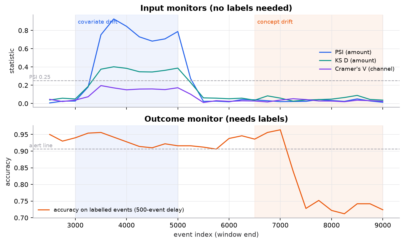
Synthetic stream. Covariate drift lights up the input monitors while accuracy barely moves. Concept drift leaves the inputs untouched and shows up only in accuracy, a window late because labels arrive 500 events after each prediction.
Try it (run drift_monitor.py, predict first, then check):
- Change the window from 500 to 200 events. Predict whether you get false alarms in the clean stretch before event 3,000.
- Set
patience=1andmin_v=0. Predict how many alerts fire in the clean stretch from 5,500 to 6,500. - Change
delayfrom 500 to 1,500. Predict the event at which the accuracy alert fires. - Add a prior-drift segment: keep the amount distribution the same but double the share of fraud. Predict which monitors react.
3. The math
Symbols
| Symbol | Meaning | Shape / range |
|---|---|---|
| , | share of reference and current values in bin | , sum to 1 |
| , | empirical CDFs of reference and current windows | |
| KS statistic | ||
| , | observed and expected count in row (window), column (category) | counts |
| total count in the contingency table | count | |
| number of categories | count | |
| Cramér's V | ||
| , | family false-alarm rate; number of tests | probability; count |
PSI
Each term is non-negative, because and always have the same sign. PSI equals the KL divergence in both directions added together. Clip zero shares to a small value (0.0001) so the log stays finite.
Worked example. Ten decile bins, so every reference share is 0.10. In the current window, bins 1 and 2 drop to 0.05 and bin 3 rises to 0.20; the rest stay at 0.10.
- Bin 1: .
- Bin 2: the same, .
- Bin 3: .
- Bins 4 to 10: .
- PSI : a moderate shift by the usual bands.
KS statistic
Worked example. Reference , current .
- At : , . Gap .
- At : , . Gap .
- At : , . Gap . No point does better, so .
The p-value depends on the effective sample size ; with large windows, tiny values become "significant", so alert on itself as well.
Chi-square and Cramér's V
with degrees of freedom.
Worked example. Channel mix (app, store, web): reference 100 events , current 100 events .
- Column totals: ; ; each row total 100.
- Expected per row: , , .
- Reference row: .
- Current row: deviations have the same size and opposite sign, so also .
- with 2 degrees of freedom, .
- : a real shift in mix, not just a significant one.
False alarms
With independent tests at level each and no real change, the expected number of false alarms is per round. 50 features checked hourly at : per hour, per day. The Bonferroni correction tests each at to keep the family rate near ; the demo uses for its two tests.
4. Implementation
Build it from scratch
The full script is code/22-ml-system-design/drift_monitor.py. NumPy for the statistics, SciPy only for the chi-square and KS p-value distributions and for checking our numbers. The stream is synthetic: 9,000 payment events with covariate drift injected at event 3,000 (bigger amounts, more app traffic), a return to normal at 5,000, and concept drift at 6,500 (the fraud boundary on amount drops from 120 to 105).
PSI on reference deciles. Bin edges come from the reference only, so each reference bin holds 10%; searchsorted assigns current values to the same bins.
def psi(reference, current, bins=10, eps=1e-4):
    edges = np.quantile(reference, np.linspace(0, 1, bins + 1)[1:-1])      # reference deciles
    e = np.bincount(np.searchsorted(edges, reference, side="right"), minlength=bins) / len(reference)
    a = np.bincount(np.searchsorted(edges, current, side="right"), minlength=bins) / len(current)
    e, a = np.maximum(e, eps), np.maximum(a, eps)                            # avoid log(0)
    return float(np.sum((a - e) * np.log(a / e)))
Predict: the current window has values far above the reference maximum. Which bin do they land in, and does PSI see how far out they are?
KS and chi-square. KS evaluates both empirical CDFs at every observed value and takes the largest gap. Chi-square builds the expected table from row and column totals.
def ks_statistic(x, y):
    """Largest vertical gap between the two empirical CDFs, evaluated at every observed value."""
    grid = np.sort(np.concatenate([x, y]))
    fx = np.searchsorted(np.sort(x), grid, side="right") / len(x)
    fy = np.searchsorted(np.sort(y), grid, side="right") / len(y)
    return float(np.max(np.abs(fx - fy)))

def chi_square(ref_counts, cur_counts):
    table = np.array([ref_counts, cur_counts], dtype=float)                 # [2, k categories]
    expected = table.sum(1, keepdims=True) * table.sum(0, keepdims=True) / table.sum()
    chi2 = float(((table - expected) ** 2 / expected).sum())
    dof = table.shape[1] - 1
    return chi2, float(stats.chi2.sf(chi2, dof)), float(np.sqrt(chi2 / table.sum()))  # Cramer's V for 2 rows
Predict: a brand-new category appears only in the current window. What happens to its expected count in the reference row, and to ?
Persistence. The policy counts consecutive drifting windows per signal and alerts only when the streak reaches patience; it reports "resolved" on the first clean window after an alert.
class Policy:
    def __init__(self, n_tests, family_alpha=0.01, psi_drift=0.25, ks_drift=0.10, min_v=0.10, patience=2):
        self.alpha, self.psi_drift, self.ks_drift, self.min_v, self.patience = family_alpha / n_tests, psi_drift, ks_drift, min_v, patience
        self.streak = {}

    def update(self, name, drifting):
        prev = self.streak.get(name, 0)
        self.streak[name] = prev + 1 if drifting else 0
        if self.streak[name] == self.patience:
            return "ALERT"
        if prev >= self.patience and not drifting:
            return "resolved"
        return None
Predict: with a sliding window that moves 250 events and is 500 long, how many events after a sudden change can the first alert fire at the earliest?
The monitoring loop. For each window: the three statistics, accuracy on the slice whose labels have arrived, and a drift flag per signal that needs both significance and effect size.
        known = slice(end - delay - window, end - delay)                     # labels only exist `delay` events back
        acc = float((pred[known] == label[known]).mean())
        flags = {"amount": p >= policy.psi_drift or (d >= policy.ks_drift and ks_p < policy.alpha),
                 "channel": chi_p < policy.alpha and v >= policy.min_v,
                 "accuracy": acc < ref_acc - tol}
Predict: at the window ending at event 3,250, the channel test has , below the per-test of 0.005, but . Does it count as drift?
Use the library
scipy.stats provides the tests directly, and the script checks its own numbers against them:
from scipy import stats
stats.ks_2samp(reference, current)              # D and an exact or asymptotic p-value
stats.chi2_contingency([ref_counts, cur_counts])  # chi2, p, dof, expected table
Monitoring tools package the statistics with storage, scheduling, and dashboards. Evidently picks a drift test per column by type and size; NannyML estimates performance before labels arrive from the model's own calibrated probabilities (which handles covariate shift but, by design, cannot see concept drift); TensorFlow Data Validation checks schema and distribution skew between training and serving. Cloud ML platforms offer the same as managed services. The from-scratch code is what each of them computes per feature; what they add is the plumbing.
Run it
uv run code/22-ml-system-design/drift_monitor.pyKey lines of output:
PSI = 0.1386
model threshold 120.8, reference accuracy 0.957
  end    PSI   KS D   chi2 p     V    acc  events
 3250  0.180  0.187  1.1e-03 0.074  0.954
 3500  0.752  0.376  1.3e-21 0.196  0.956  ALERT amount
 3750  0.926  0.402  1.4e-16 0.171  0.942  ALERT channel
 5500  0.024  0.061  8.6e-01 0.011  0.912  resolved amount, resolved channel
 7500  0.023  0.039  9.7e-02 0.043  0.728  ALERT accuracy
scratch KS D = 0.3850;  scipy ks_2samp D = 0.3850
scratch chi2 = 56.08;  scipy chi2_contingency = 56.08
Read it in three parts. Covariate drift starts at 3,000; the amount alert fires at 3,500 and accuracy stays above 0.9 because the fraud rule did not change. Inputs return to normal at 5,000 and both alerts resolve at 5,500. Concept drift starts at 6,500; the input monitors stay quiet, and the accuracy alert fires at 7,500, 1,000 events later, of which 500 are the label delay.
5. Engineering
Monitor what matters most. You cannot alert on every feature. Rank features by importance to the model and by how likely they are to break (upstream joins, third-party sources), watch the top ones closely, and summarize the rest. Always watch the prediction distribution: it is one signal that integrates all inputs.
Catch pipeline bugs first. Most "drift" in practice is a broken pipeline: a unit change (dollars to cents), a column filled with defaults, a renamed category, a feature computed differently online than offline (training-serving skew). Schema checks, missing-value rates, and range checks catch these cheaply and should page faster than statistical drift.
Get labels sooner. Use fast proxies (early chargebacks, first-week engagement), label a random sample by hand, or join delayed labels as soon as they land and compute outcome metrics on that slice. Track calibration as well as accuracy.
Decide the action by drift type.
| Finding | Action |
|---|---|
| Pipeline bug | fix the pipeline; do not retrain on broken data |
| Covariate drift, outcomes stable | usually none; keep watching outcomes |
| Covariate drift into sparse regions | retrain with recent data covering those regions |
| Prior drift | recalibrate scores or thresholds to the new base rate |
| Concept drift | collect recent labels and retrain; old labels teach the old concept |
Retraining triggers. Schedules are simple but retrain when nothing changed and wait when something did. Drift- or performance-triggered retraining reacts to evidence. Either way, validate the new model on the most recent labelled data, roll it out through shadow and canary stages, and reset the reference window afterwards.
Feedback loops. When the model's decisions control which labels you see (rejected loans never default, blocked transactions never charge back), outcome metrics are biased. Keep a small randomized holdout, as in experimentation, to measure the truth.
Per-group monitoring. Aggregate metrics can be stable while one segment degrades. Track key metrics per region, platform, and, where relevant, per protected group (see Fairness).
Watch outFailure modes. Alerting on p-values alone with large windows; dozens of uncorrected tests and an ignored alert channel; no outcome monitoring, so concept drift goes unseen; a reference window that is itself unrepresentative; seasonality read as drift; retraining on data from a broken pipeline; and dashboards nobody owns.
Common mistakes
- Monitoring only latency and errors, and calling the model "healthy".
- Treating PSI bands as a statistical test.
- Using a reference window from a different season, then chasing weekly cycles.
- Retraining automatically on any drift, including drift caused by an upstream bug.
- Measuring accuracy on all predictions, including those whose labels haven't arrived.
- Forgetting to reset the reference after retraining, so every later window looks drifted.
6. Knowledge check
Quiz: Model monitoring and drift
Which monitoring layer is the only one that directly measures whether the model is still correct?
Practice exercise. A feature is binned into five reference quintiles (0.20 each). The current window's shares are . Compute PSI and classify it with the usual bands.
Solution
- .
- .
- .
- .
- .
PSI : a moderate shift (between 0.1 and 0.25). The mass has moved toward higher values.
Implementation challenge. Add a prediction monitor to drift_monitor.py: track the model's positive-prediction rate per window and alert when it moves more than 5 percentage points from the reference rate for two windows in a row. Which drift period does it catch, and why does it miss the other?
Solution sketch
Compute ref_pos = pred[:ref_size].mean() and, per window, pos = pred[cur].mean(); flag abs(pos - ref_pos) > 0.05 and pass it through policy.update("positive_rate", ...). It fires during covariate drift, because bigger amounts push more predictions over the fixed threshold. It stays quiet during concept drift, because the model's inputs (and therefore its predictions) are unchanged; only the true labels moved. Prediction monitors integrate input drift; they cannot see concept drift any more than input monitors can.
Summary
- Monitor four layers: system, inputs, predictions (all immediate), and outcomes (delayed by labels).
- Covariate drift changes , prior drift , concept drift ; only outcome monitoring sees concept drift.
- PSI compares binned shares, KS takes the largest CDF gap, chi-square with Cramér's V handles categories; use effect sizes, not just p-values.
- Alert policies need multiple-testing correction, effect-size thresholds, and persistence, or people stop reading them.
- Match the action to the cause: fix pipelines, recalibrate for prior drift, retrain with fresh labels for concept drift, and reset the reference after retraining.
Next: The 12-week plan
Related: ML system design · Experimentation and A/B testing · Reliability, cost, and observability · Fairness
Parts of this lesson are adapted from AI Engineering from Scratch by Rohit Ghumare (MIT license, notice): Monitoring Models in Production — Data Drift and Concept Drift.
Interview angle
How would you monitor a fraud model after deployment?
In four layers. System health: latency, error rate, throughput, so the service answers. Inputs: for the most important features, PSI or KS against the training window, plus missing rates, schema checks, and new categories, because most incidents are pipeline bugs. Predictions: the score distribution and the share of transactions flagged, which reacts to almost any input change. Outcomes: precision, recall, and calibration on transactions whose chargebacks have arrived, which can take weeks, so I'd add faster proxies like early disputes and a manually reviewed sample. Alerts use Bonferroni-corrected thresholds, require an effect size, and need two consecutive windows. Because the model blocks transactions, blocked ones never charge back, so I'd keep a tiny randomized holdout to measure true fraud rates. And I'd break metrics down by region and channel.
What's the difference between covariate drift and concept drift, and why does it matter for what you do next?
Covariate drift is a change in the input distribution, P of x, while the relationship between inputs and the label stays the same. Concept drift is a change in that relationship, P of y given x: the same input now has a different correct answer. It matters because the monitors and the fixes differ. Input monitors like PSI catch covariate drift immediately, and often no action is needed if the model was right across those inputs; you retrain only if traffic moved into regions with little training data. Concept drift leaves the inputs looking normal, so only outcome metrics reveal it, after the label delay. Retraining on old labels doesn't help, because they encode the old concept; you need fresh labels. A third case, prior drift, where the base rate changes, is often fixed by recalibrating thresholds.
Your drift dashboard pages the team several times a day and people have started ignoring it. What do you change?
First I'd count where the pages come from. Usually it's three things. Too many uncorrected tests: 50 features checked hourly at 0.05 gives about 60 false alarms a day with no real change, so I'd apply a Bonferroni or false-discovery-rate correction. P-values without effect sizes: with big windows, tiny shifts are significant, so I'd require PSI above 0.25, KS D above 0.1, or Cramér's V above 0.1 as well. No persistence: one noisy window shouldn't page anyone, so I'd require two or three in a row. Then I'd check seasonality, comparing Monday with last Monday. Finally, split warnings from alerts: warnings go to a dashboard, and only drift on important features, schema breaks, or outcome drops page a person, each with an owner and a runbook.
Ten reference deciles; in the current window, two bins drop to 5% and one rises to 20%. What's the PSI, and is it worth an alert?
PSI sums current share minus reference share, times the log of their ratio, over bins. The two bins at 5% each contribute minus 0.05 times ln 0.5, which is 0.05 times 0.693, about 0.035. The bin at 20% contributes 0.10 times ln 2, about 0.069. The unchanged bins add zero. Total: 0.035 plus 0.035 plus 0.069, about 0.139. By the usual credit-scoring bands that's a moderate shift: above 0.1, below 0.25. I wouldn't page on it alone. I'd log a warning, check whether it persists over the next window or two, look at whether the feature matters to the model and whether the prediction distribution moved, and check outcome metrics as labels arrive. If it persists and the feature is important, it's worth investigating.