Support vector machines

Quick read: the intuition, interactive visualization, summary, and interview questions. The math, implementation, engineering, and knowledge-check sections are hidden.

Mental model. Of all the lines that separate two classes, choose the one with the widest empty street around it. Only the points on the edge of the street (the support vectors) decide where it goes. Kernels let the street curve.

You will learn to

Define the margin and support vectors, and compute the margin width from the weights.
Explain the soft-margin trade-off controlled by C.
Write the hinge loss and compare it with logistic loss.
Explain the kernel trick and the RBF kernel's $\gamma$ parameter.
Decide when an SVM is a good choice in practice.

Why it matters. Linear SVMs are excellent on high-dimensional sparse data like TF-IDF text. Kernel SVMs dominated many benchmarks before deep learning and remain strong on small and medium datasets. The margin idea also explains why some models generalize better than others that fit the training data equally well.

1. Intuition

Many lines can separate two well-separated groups. A line that barely squeezes past some points will misclassify new points that land slightly off. A line with a wide buffer on both sides is more robust. The SVM maximizes that buffer, the margin.

Real data overlaps, so a soft margin allows some points inside the street or on the wrong side, at a cost. The hyperparameter C sets the price: large C insists on classifying training points correctly (narrow street, risk of overfitting); small C accepts some errors for a wider street (smoother, more regularized).

When no straight line works, the kernel trick computes similarities as if the data had been mapped into a richer feature space where a linear separator exists, without ever building that space explicitly.

2. Visualization

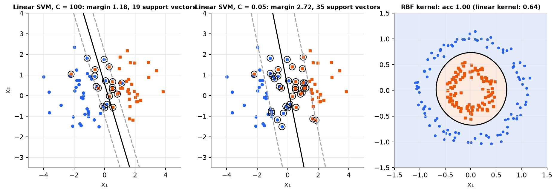
Left: a linear SVM with C = 100 has a narrow margin (dashed lines) and 19 circled support vectors. Middle: C = 0.05 has a margin more than twice as wide with 35 support vectors. Right: on two concentric rings, an RBF-kernel SVM draws a circular boundary with 100% accuracy where a linear kernel gets 64%.

Synthetic data. Both linear models reach the same training accuracy (0.925); the wider margin is the more regularized choice.

3. The math

Symbols

Symbol	Meaning
$y_i \in \{-1, +1\}$	labels (SVMs use ±1)
$w, b$	boundary $w \cdot x + b = 0$
$\xi_i \ge 0$	slack: how far point $i$ violates the margin
$C$	penalty per unit of slack
$K(x, x')$	kernel: similarity between two points
$\gamma$	RBF kernel width parameter

Hard margin

The margin edges are $w\cdot x + b = \pm 1$ . The distance between them is $2/\lVert w \rVert$ , so maximizing the margin means minimizing $\lVert w \rVert$ :

\min_{w,b} \tfrac12\lVert w\rVert^2 \quad \text{subject to} \quad y_i(w\cdot x_i + b) \ge 1 \;\text{for all } i

Soft margin and hinge loss

\min_{w,b} \tfrac12\lVert w\rVert^2 + C\sum_i \xi_i \;\;\Longleftrightarrow\;\; \min_{w,b} \tfrac12\lVert w\rVert^2 + C\sum_i \max\big(0,\; 1 - y_i(w\cdot x_i + b)\big)

The hinge loss $\max(0, 1 - y\,f(x))$ is zero for points correctly classified beyond the margin, so they have no influence. That is why only support vectors matter.

Kernels

The solution depends on the data only through dot products $x_i \cdot x_j$ . Replacing them with a kernel gives a nonlinear boundary:

f(x) = \sum_{i \in \text{SV}} \alpha_i y_i K(x_i, x) + b, \qquad K_{\text{RBF}}(x, x') = \exp\!\big(-\gamma\lVert x - x'\rVert^2\big)

Large $\gamma$ : each support vector influences only its immediate neighborhood (wiggly boundary, overfitting risk). Small $\gamma$ : smooth boundary.

Worked example

A trained linear SVM has $w = (3, 4)$ and $b = -2$ .

Margin width: $2/\lVert w \rVert = 2/\sqrt{9 + 16} = 2/5 = 0.4$ .
Point $x = (1, 0.5)$ with $y = +1$ : $f(x) = 3 + 2 - 2 = 3$ . $y f(x) = 3 \ge 1$ , so it is outside the margin: hinge loss 0, not a support vector.
Point $x = (0.2, 0.3)$ with $y = +1$ : $f(x) = 0.6 + 1.2 - 2 = -0.2$ . $y f(x) = -0.2$ : misclassified, hinge loss $= 1 - (-0.2) = 1.2$ .
RBF similarity between $(0, 0)$ and $(1, 1)$ with $\gamma = 0.5$ : $\exp(-0.5 \times 2) = e^{-1} = 0.368$ .

4. Implementation

Build it from scratch

The full script is code/05-instance-and-probabilistic/svm_scratch.py. It trains a linear SVM with plain NumPy by subgradient descent on the soft-margin objective, then checks it against scikit-learn. Production solvers use the dual form or coordinate descent instead, but they minimize the same objective.

Hinge loss and the objective. Each point pays $\max(0, 1 - y_i f(x_i))$ . Points with $y_i f(x_i) \ge 1$ sit outside the street and pay nothing; points inside the street or on the wrong side pay linearly. We write the soft margin as $\frac{\lambda}{2}\lVert w\rVert^2 + \frac{1}{n}\sum_i \text{hinge}_i$ . This is the section 3 objective divided by $Cn$ , so it has the same minimizer when $C = 1/(\lambda n)$ : large $\lambda$ means small $C$ , a wider street with more violations.

python

def hinge(X, y, w, b):
    margins = y * (X @ w + b)                  # y_i f(x_i): >= 1 means safely outside the street
    return np.maximum(0.0, 1.0 - margins)      # [n], zero for points beyond the margin

def objective(X, y, w, b, lam):                # lambda/2 ||w||^2 + mean hinge
    return 0.5 * lam * w @ w + hinge(X, y, w, b).mean()

Predict: a correctly classified point has $y f(x) = 0.5$ . What is its hinge loss? And if you multiply $\lambda$ by 10, does the margin width $2/\lVert w\rVert$ grow or shrink?

The script's first print applies hinge to the two points of the worked example in section 3 ( $w = (3, 4)$ , $b = -2$ ).

One subgradient step. The hinge has a corner at $y f(x) = 1$ , so we use a subgradient. Points outside the margin contribute zero gradient; only the "active" violators pull on $w$ and $b$ . The regularizer shrinks $w$ every step. This is the support-vector idea in code: points that never become active never affect the answer.

python

def step(X, y, w, b, lam, lr):
    active = y * (X @ w + b) < 1               # only margin violators push on w and b
    grad_w = lam * w - (y[active, None] * X[active]).sum(axis=0) / len(y)
    grad_b = -y[active].sum() / len(y)
    return w - lr * grad_w, b - lr * grad_b

Predict: you delete a training point that ends far outside the margin and retrain. Does the boundary move?

Train. Repeat the step with a learning rate that decays as $1/\sqrt{t}$ . A fixed step would bounce around the corner of the hinge forever; the decay lets it settle. Labels must be $\pm 1$ , so the script converts scikit-learn's $\{0, 1\}$ with 2 * y01 - 1.

python

def fit_linear_svm(X, y, lam=0.01, lr=0.5, epochs=3000):
    w, b = np.zeros(X.shape[1]), 0.0
    for t in range(epochs):
        w, b = step(X, y, w, b, lam, lr / np.sqrt(1 + t))   # decaying step for a non-smooth loss
    return w, b

Predict: if you forget the label conversion and train on $\{0, 1\}$ , what do the class-0 points contribute to grad_w?

The RBF kernel matrix. A kernel SVM never builds features; it needs only pairwise similarities. Expanding $\lVert a - b\rVert^2 = \lVert a\rVert^2 + \lVert b\rVert^2 - 2a\cdot b$ computes all pairs with one matrix product. Clipping at 0 removes tiny negative values from floating-point rounding.

python

def rbf_kernel(A, B, gamma=0.5):
    sq = (A**2).sum(1)[:, None] + (B**2).sum(1)[None, :] - 2 * A @ B.T   # ||a - b||^2 for all pairs
    return np.exp(-gamma * np.maximum(sq, 0.0))

K = rbf_kernel(np.array([[0.0, 0.0], [1.0, 1.0], [3.0, 3.0]]), np.array([[0.0, 0.0]]))
print(f"\nRBF similarity to (0,0), gamma=0.5: {K.ravel().round(4)}")

Predict: the kernel matrix for $n$ training points has how many entries? At $n = 100{,}000$ in float64, about how many gigabytes is that?

Use the library

python

from sklearn.model_selection import GridSearchCV
from sklearn.pipeline import make_pipeline
from sklearn.preprocessing import StandardScaler
from sklearn.svm import SVC, LinearSVC

# Linear SVM: fast on large sparse data (e.g. TF-IDF)
text_clf = make_pipeline(TfidfVectorizer(), LinearSVC(C=1.0))

# RBF SVM: tune C and gamma together, always with scaling
rbf = make_pipeline(StandardScaler(), SVC(kernel="rbf"))
search = GridSearchCV(rbf, {"svc__C": [0.1, 1, 10, 100], "svc__gamma": [0.01, 0.1, 1]}, cv=5)
search.fit(X_train, y_train)

TfidfVectorizer comes from sklearn.feature_extraction.text.

Scratch	scikit-learn
`fit_linear_svm(..., lam=)`	`SVC(kernel="linear", C=1/(lam*n))`; `LinearSVC(C=)` for large data
`w`, `b`	`coef_`, `intercept_`
points with `y * f(x) <= 1`	`support_`, `support_vectors_`
`rbf_kernel(..., gamma=)`	`SVC(kernel="rbf", gamma=)`

One difference: LinearSVC by default uses the squared hinge and also regularizes the intercept, so its weights differ slightly from SVC(kernel="linear"). The script compares against SVC, which minimizes exactly our objective.

Run it

From guide/:

bash

uv run code/05-instance-and-probabilistic/svm_scratch.py

Key output:

text

worked example: margin width 0.40, hinge losses [0.  1.2]

scratch: w=[1.439 0.334] b=0.042  objective 0.1531  train acc 0.935
sklearn: w=[1.439 0.334] b=0.042  objective 0.1531  train acc 0.935  support vectors 35

RBF similarity to (0,0), gamma=0.5: [1.000e+00 3.679e-01 1.000e-04]

On this synthetic data the scratch weights match scikit-learn's to three decimals. The RBF line matches the worked example: $e^{-0.5 \times 2} = 0.368$ for $(1, 1)$ , and $e^{-0.5 \times 18} \approx 0.0001$ for $(3, 3)$ . The figure script is code/05-instance-and-probabilistic/nb_svm.py.

5. Engineering

Good fits. Text classification with TF-IDF (linear SVM); small-to-medium datasets with complex boundaries (RBF); high-dimensional data where $p > n$ .

Poor fits. Very large $n$ for kernel SVMs: training scales between $O(n^2)$ and $O(n^3)$ and memory holds a kernel matrix. Use linear SVMs, approximate kernels, or gradient boosting instead.

Preprocessing. Scale features; SVMs use distances and dot products.

Probabilities. SVM outputs are margins, not probabilities. SVC(probability=True) fits a calibration step with extra cross-validation; or use CalibratedClassifierCV.

Watch out
Failure modes. Unscaled features; untuned C and γ (defaults are rarely right); kernel SVMs on hundreds of thousands of rows; treating decision-function values as probabilities.

Common mistakes

Tuning C without tuning γ (they interact).
Using an RBF kernel on sparse text where linear works better and is much faster.
Expecting interpretable weights from a kernel SVM.

6. Knowledge check

Quiz: Support vector machines

Question 1 of 6

Calculationmedium

A linear SVM has $w = (6, 8)$ . What is the margin width $2/\lVert w\rVert$ ?

Practice exercise. With $w = (1, -1)$ and $b = 0$ , compute the margin width and the hinge loss for $x = (2, 1.5)$ , $y = +1$ .

Solution

$\lVert w \rVert = \sqrt{2} = 1.414$ , so the margin is $2/1.414 = 1.414$ . $f(x) = 2 - 1.5 = 0.5$ ; $y f(x) = 0.5 < 1$ , so hinge loss $= 1 - 0.5 = 0.5$ : correctly classified but inside the margin, so it is a support vector.

Implementation challenge. Implement a linear SVM with subgradient descent on the hinge loss plus $\frac{\lambda}{2}\lVert w\rVert^2$ and compare its accuracy and weights with LinearSVC.

Summary

SVMs maximize the margin $2/\lVert w\rVert$ between classes; only support vectors define the boundary.
C trades margin width against training errors; hinge loss ignores well-classified points.
Kernels (RBF with width γ) give nonlinear boundaries using only pairwise similarities.
Linear SVMs shine on sparse text; kernel SVMs don't scale to very large datasets; scale features and calibrate if you need probabilities.

Next: Decision trees

Go deeper, code-first (AI Engineering from Scratch): Convex Optimization

Parts of this lesson are adapted from AI Engineering from Scratch by Rohit Ghumare (MIT license, notice): Support Vector Machines.

Interview angle

What are support vectors, and why do only they determine the SVM?

Support vectors are the training points on or inside the margin, or misclassified: those with $y_i(w \cdot x_i + b) \le 1$ . The hinge loss $\max(0, 1 - y_i f(x_i))$ is exactly zero for every point correctly classified beyond the margin, so those points contribute nothing to the objective or its gradient. You could move or delete them, as long as they don't cross the margin, and the solution wouldn't change. The dual form makes this explicit: $f(x) = \sum_{i \in \text{SV}} \alpha_i y_i K(x_i, x) + b$ , with $\alpha_i = 0$ for every non-support vector. Consequences: the model is defined by a subset of the data; prediction cost scales with the number of support vectors; and a large fraction of support vectors, from small $C$ or heavily overlapping classes, means slow prediction and hints that the classes are hard to separate.

Explain the kernel trick. Why not just compute the expanded features explicitly?

The SVM solution depends on the data only through dot products $x_i \cdot x_j$ . A kernel $K(x, x')$ computes a dot product $\phi(x) \cdot \phi(x')$ in some feature space without ever constructing $\phi$ . A degree-3 polynomial kernel on $p = 1000$ features corresponds to roughly $1.7 \times 10^8$ monomial features, yet $(x \cdot x' + 1)^3$ costs only $O(p)$ . The RBF kernel $\exp(-\gamma\lVert x - x'\rVert^2)$ corresponds to an infinite-dimensional feature space, which can't be built explicitly at all. The cost moves elsewhere: the kernel matrix is $n \times n$ , so training scales roughly between $O(n^2)$ and $O(n^3)$ , and each prediction needs a kernel evaluation against every support vector. For large $n$ , approximate the feature map instead (random Fourier features, Nyström) and train a fast linear model on it.

Your RBF SVM gets 100% training accuracy and 60% test accuracy. What do you tune?

That's overfitting, and in an RBF SVM it usually comes from $\gamma$ too large, $C$ too large, or both. A large $\gamma$ makes each support vector's influence very local, so the boundary wraps around individual training points; a quick check is whether nearly every training point is a support vector. A large $C$ penalizes every margin violation heavily, so the model contorts itself to classify noisy points. Fix: search $C$ and $\gamma$ jointly on a log grid (say $10^{-3}$ to $10^{3}$ ) with cross-validation, because they interact: a smaller $\gamma$ often wants a larger $C$ . Also confirm features were scaled: RBF distances on unscaled data are dominated by one feature, and the default gamma="scale" assumes comparable feature scales. For high-dimensional sparse text, try a linear kernel first; it's often both more accurate and much faster.

A linear SVM has w = (3, 4) and b = -2. What's the margin width, how far is x = (1, 0.5) from the boundary, and what changes if you double w and b?

Margin width $= 2/\lVert w \rVert = 2/5 = 0.4$ . At $x = (1, 0.5)$ , the functional value is $f(x) = 3 + 2 - 2 = 3$ , and the geometric distance to the boundary is $|f(x)|/\lVert w \rVert = 3/5 = 0.6$ , so the point sits 0.4 beyond the margin edge, which is 0.2 from the boundary. Doubling to $w = (6, 8)$ , $b = -4$ leaves the boundary $w \cdot x + b = 0$ unchanged, but $f(x)$ becomes 6 and the margin edges $f = \pm 1$ move closer: the width drops to $2/10 = 0.2$ . That's why the SVM fixes the scale with the constraint $y_i f(x_i) \ge 1$ and minimizes $\lVert w \rVert$ : otherwise functional margins could be inflated for free. It's also why raw decision-function values aren't probabilities and aren't comparable across models.