Module 10: Neural-network foundations 50 min11 min quick readDeep learning
Intro to PyTorch
Build a tiny autograd engine, then use PyTorch tensors, autograd, nn.Module, and the five-line training loop to train a network on CPU, and recognize the bugs that loop invites.
Before this: Loss functions, Backpropagation, The Python toolkit
Quick read: the intuition, interactive visualization, summary, and interview questions. The math, implementation, engineering, and knowledge-check sections are hidden.
Mental model. PyTorch is NumPy that keeps a receipt. Every operation on a tensor that needs gradients is written onto a receipt (the computational graph). When you call
loss.backward(), PyTorch reads the receipt backwards and applies the chain rule at each line, filling in.gradfor every parameter. Everything else (layers, optimizers, data loaders) is convenience built on that one idea.
You will learn to
- Build a scalar autograd engine and check its gradients against PyTorch.
- Create and reshape tensors, and predict shapes, dtypes, and broadcasting results.
- Explain
requires_grad,.backward(), gradient accumulation, andtorch.no_grad(). - Define a model with
nn.Moduleand count its parameters. - Write the training loop (forward, loss, zero_grad, backward, step) and the evaluation loop, and say what
model.train()andmodel.eval()change.
Why it matters. PyTorch is the default framework for deep-learning research and most production training, and the Hugging Face ecosystem is built on it. Coding interviews for ML roles often ask you to write a training loop from memory, and the most common bugs (forgetting zero_grad, forgetting eval(), applying softmax before the loss) all live in about ten lines. Knowing what autograd actually does makes those bugs obvious.
1. Intuition
In backpropagation you computed gradients by hand: run the forward pass, then walk backwards multiplying local derivatives. That is mechanical, so a computer can do it if it remembers what happened.
PyTorch remembers. A tensor is an n-dimensional array, like a NumPy array, that can live on a CPU or GPU. If a tensor has requires_grad=True (all model parameters do), every operation on it creates a new tensor that records which operation made it and from which inputs. Chained together, these records form a graph from the parameters to the loss.
loss.backward() walks that graph from the loss back to the parameters. At each node it applies that operation's local derivative, multiplies by the gradient flowing in (the chain rule), and adds the result into the inputs' .grad. Note the word adds: gradients accumulate. That's handy (you can sum gradients over several small batches) and dangerous (if you forget to reset them, each step uses the sum of all previous gradients).
On top of autograd:
nn.Moduleis a container that registers its parameters, somodel.parameters()finds them all.- An optimizer (SGD, AdamW) holds references to those parameters and, on
step(), updates each one using its.grad. - A
DataLoadercuts the dataset into shuffled mini-batches.
The training loop is the same five steps every time: forward, loss, clear old gradients, backward, step.
2. Visualization
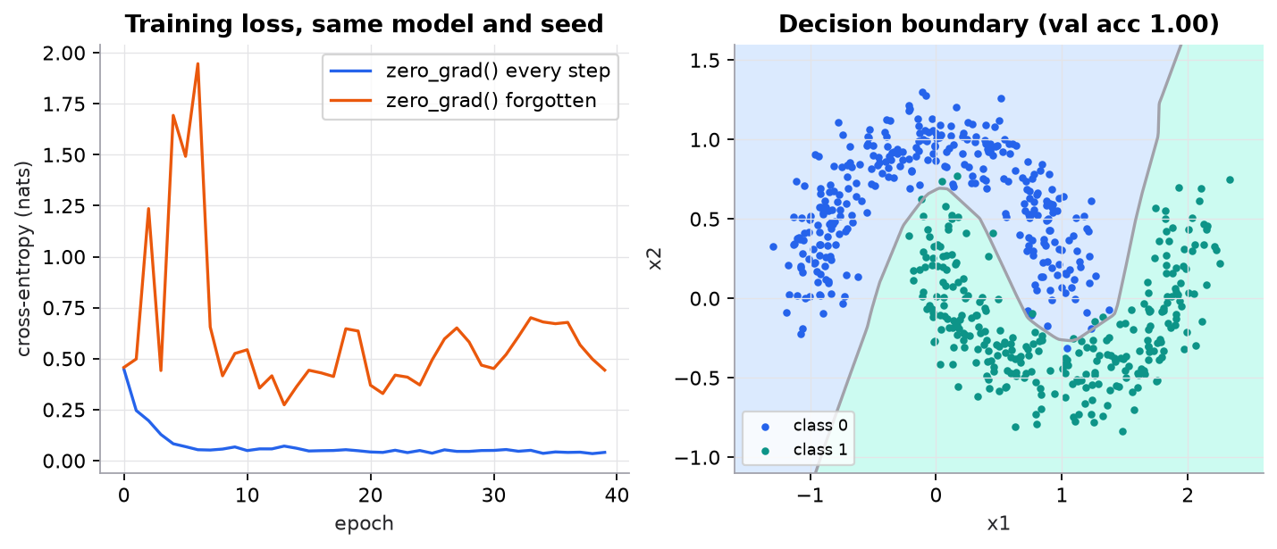
Synthetic two-moons data, 480 training and 120 validation points. Left: one missing line (opt.zero_grad()) and every step uses the running sum of all earlier gradients. Right: what the correct loop learned, a curved boundary no linear model could draw.
Try it (predict, then run the script):
- Without
zero_grad, the effective gradient is a sum that keeps growing. AdamW divides by a running estimate of gradient size, which partly hides this. Predict what happens if you switch the optimizer to plaintorch.optim.SGD(..., lr=0.1). - Remove
model.eval()fromaccuracy. Predict whether validation accuracy changes from run to run, and why. - Change
hidden=32tohidden=4. Predict the new parameter count before running. - Print
model(xtr).shapeandytr.shape. Why doesF.cross_entropyaccept a[480, 2]float tensor and a[480]integer tensor?
3. The math
This lesson is about a mechanism, so this section walks one tiny computation through autograd with every number.
Symbols
| Symbol | Meaning | Shape |
|---|---|---|
| input | scalar here; in a model | |
parameters (requires_grad=True) | scalars here | |
| prediction | scalar | |
| target | scalar | |
| loss | scalar | |
the gradient stored in v.grad | same shape as | |
| learning rate | scalar |
Forward pass: build the graph
With , , , , autograd records four nodes:
| Node | Operation | Value | Local derivatives |
|---|---|---|---|
| , | |||
Backward pass: walk it in reverse
Start with . Each step multiplies the incoming gradient by the local derivative:
So w.grad = -12 and b.grad = -6, which both the scratch engine and PyTorch print.
Accumulation and the update
Call backward again on a freshly computed loss without clearing, and each .grad gets the new gradient added: . That's what zero_grad() prevents.
One SGD step with and the correct gradients:
New prediction , new loss , down from 9.
Shapes in the real model
The script's MLP maps . nn.Linear(in, out) stores a weight of shape and computes . Parameters:
F.cross_entropy(logits, y) takes logits (float) and class indices (int64), and returns the mean loss, a scalar, which is what .backward() needs. At step 0 it should be near for 2 classes; the script prints 0.682.
4. Implementation
Build it from scratch
A Value holds a number, its gradient, the values it came from, and a function that pushes its gradient to those parents. Addition and multiplication each record their local derivatives.
class Value:
    """A number that remembers how it was computed, so it can send gradients back."""

    def __init__(self, data, parents=(), backward=lambda: None):
        self.data, self.grad = data, 0.0
        self._parents, self._backward = parents, backward

    def __add__(self, other):
        other = other if isinstance(other, Value) else Value(other)
        out = Value(self.data + other.data, (self, other))
        def backward():                       # d(a+b)/da = 1, d(a+b)/db = 1
            self.grad += out.grad
            other.grad += out.grad
        out._backward = backward
        return out
Predict: why += rather than = in backward? (Hint: what if the same value is used twice, as in a + a?)
Multiplication swaps in the other factor; power uses the power rule. Subtraction is built from the other two.
    def __mul__(self, other):
        other = other if isinstance(other, Value) else Value(other)
        out = Value(self.data * other.data, (self, other))
        def backward():                       # d(ab)/da = b, d(ab)/db = a
            self.grad += other.data * out.grad
            other.grad += self.data * out.grad
        out._backward = backward
        return out

    def __sub__(self, other):
        return self + (other * -1 if isinstance(other, Value) else -other)

    def __pow__(self, k):
        out = Value(self.data**k, (self,))
        def backward():                       # d(a^k)/da = k a^(k-1)
            self.grad += k * self.data ** (k - 1) * out.grad
        out._backward = backward
        return out
Predict: for c = a * b with a = 3, b = 2, and c.grad = 1, what are a.grad and b.grad?
backward() sorts the graph so each node runs after every node that uses it, seeds the loss with gradient 1, and walks in reverse.
    def backward(self):
        order, seen = [], set()
        def visit(v):                         # topological order: parents before children
            if v not in seen:
                seen.add(v)
                for p in v._parents:
                    visit(p)
                order.append(v)
        visit(self)
        self.grad = 1.0                       # dL/dL = 1
        for v in reversed(order):             # walk from the loss back to the leaves
            v._backward()
Predict: what goes wrong if you call L.backward() twice on the same L? (Every intermediate .grad still holds its first-pass value, so the second pass adds on top at every node: w.grad ends at −60, not −24. PyTorch frees the graph after backward(), so a second call raises an error unless you pass retain_graph=True.)
That is all of autograd. PyTorch does the same thing on tensors, with each operation's backward written in C++ or CUDA.
Use the library
Same graph, same numbers:
wt = torch.tensor(3.0, requires_grad=True)
bt = torch.tensor(1.0, requires_grad=True)
Lt = (wt * 2.0 + bt - 10.0) ** 2
Lt.backward()                                # wt.grad = -12, bt.grad = -6
A model is an nn.Module. Layers assigned as attributes are registered, so model.parameters() finds their weights. The last layer outputs raw logits, because F.cross_entropy applies log-softmax itself (see loss functions).
class MLP(nn.Module):
    def __init__(self, d_in=2, hidden=32, d_out=2):
        super().__init__()
        self.net = nn.Sequential(
            nn.Linear(d_in, hidden), nn.ReLU(),
            nn.Linear(hidden, hidden), nn.ReLU(),
            nn.Dropout(0.1),
            nn.Linear(hidden, d_out),           # raw logits: no softmax here
        )

    def forward(self, x):                       # x: [batch, d_in] -> logits: [batch, d_out]
        return self.net(x)
The training loop, five numbered steps. model.train() turns dropout (and batch-norm statistics updates) on.
def train(model, loader, epochs, lr=1e-2, zero_grad=True):
    opt = torch.optim.AdamW(model.parameters(), lr=lr)
    losses = []
    for _ in range(epochs):
        model.train()                           # dropout on
        total = 0.0
        for xb, yb in loader:
            logits = model(xb)                  # 1. forward
            loss = F.cross_entropy(logits, yb)  # 2. loss
            if zero_grad:
                opt.zero_grad()                 # 3. clear old gradients
            loss.backward()                     # 4. backward: fill .grad
            opt.step()                          # 5. update parameters
            total += loss.item() * len(xb)
        losses.append(total / len(loader.dataset))
    return losses
Evaluation turns off both dropout (model.eval()) and graph recording (torch.no_grad(), here as a decorator), which saves memory and time.
@torch.no_grad()
def accuracy(model, x, y):
    model.eval()                                # dropout off
    return (model(x).argmax(1) == y).float().mean().item()
.item() pulls a Python number out of a one-element tensor; use it for logging so you don't keep the graph alive by storing the loss tensor. Save weights with torch.save(model.state_dict(), path) and restore with model.load_state_dict(torch.load(path, weights_only=True)).
Beyond CPU. Move the model and every batch to the same device: device = "cuda" if torch.cuda.is_available() else "cpu", then model.to(device) and xb.to(device) (Apple silicon uses "mps"). torch.compile(model) (PyTorch 2.x) traces and fuses the model into faster kernels without changing your code; for real training add mixed precision with torch.autocast (see numerical stability).
Run it
uv run code/10-neural-networks/intro_to_pytorch.pyPyTorch is declared in the script's header (PEP 723 inline metadata), so uv installs it into a cached environment on first run; that download takes a minute or two. Key output:
L = 9.0, dL/dw = -12.0, dL/db = -6.0
L = 9.0, dL/dw = -12.0, dL/db = -6.0
after a second backward without zeroing: dL/dw = -24.0 (gradients accumulate)
X + bias =
tensor([[10., 21., 32.],
        [13., 24., 35.]])
weight (3, 2), bias (3,)  (out_features, in_features)
parameters: 1218  (2*32+32 + 32*32+32 + 32*2+2)
step-0 loss 0.6815 (ln 2 = 0.6931)
correct loop:      final train loss 0.0406, val accuracy 1.000
no zero_grad():    final train loss 0.4439, val accuracy 0.775
train mode, same input twice -> identical? False;  eval mode -> identical? True
Exact losses can differ slightly across PyTorch versions and CPUs; the pattern won't.
5. Engineering
Where the time goes. PyTorch is fast because each tensor operation runs as one optimized kernel over the whole batch. Python loops over individual numbers (like the scratch Value) are millions of times slower. Keep work in batched tensor ops, and keep the GPU busy: DataLoader(num_workers=..., pin_memory=True) overlaps data loading with compute.
Memory. Autograd keeps every intermediate activation until backward, so activation memory grows with batch size and depth. Use torch.no_grad() (or torch.inference_mode()) for evaluation, and gradient checkpointing for very deep models. Accumulating total += loss (a tensor) instead of loss.item() keeps every step's graph alive and leaks memory.
Reproducibility. Seed torch.manual_seed, the DataLoader's generator, and NumPy/Python if used. On GPU, some kernels are non-deterministic; torch.use_deterministic_algorithms(True) trades speed for repeatability.
Gradient accumulation on purpose. To simulate a batch of 256 on a GPU that fits 64, call backward() on loss / 4 for four micro-batches, then step() and zero_grad() once. This is the useful side of accumulation.
Checkpoints. Save model.state_dict(), optimizer.state_dict(), the scheduler, the step, and the RNG states, so a resumed run continues exactly. Load with weights_only=True for files you didn't create; arbitrary pickles can run code.
Watch outFailure modes. Forgetting
opt.zero_grad()(gradients accumulate across steps); forgettingmodel.eval()(dropout stays on and batch norm uses batch statistics at inference); softmax beforeF.cross_entropy; model on GPU and data on CPU (a device mismatch error); calling.numpy()on a tensor that requires grad (use.detach()first); in-place operations on tensors autograd still needs.
Common mistakes
- Putting
zero_grad()in the wrong place (it must run before eachbackward(), not betweenbackward()andstep()). - Thinking
torch.no_grad()andmodel.eval()do the same thing. One stops graph recording; the other changes layer behaviour. Inference needs both. - Using integer tensors as model inputs (
torch.arange(6)is int64;nn.Linearneeds float). - Leaving
shuffle=Trueon the validation loader and then comparing per-batch metrics across runs.
6. Knowledge check
Quiz: Intro to PyTorch
What is autograd in PyTorch?
Practice exercise. With , , , , compute and both gradients by hand. Then compute and after one SGD step with .
Solution
. . .
. . .
Update: ; . New prediction , new loss .
Implementation challenge. Add a relu() method to Value, build a 2-input neuron , and check all three gradients against PyTorch for one input where the ReLU is active and one where it is not.
Solution
def relu(self):
    out = Value(max(0.0, self.data), (self,))
    def backward():
        self.grad += (self.data > 0) * out.grad      # slope 1 if active, else 0
    out._backward = backward
    return out
Value.relu = relu
For an active input, each weight's gradient is its input and the bias gradient is 1 (times the upstream gradient). For an inactive input, all three are 0, in both engines. That zero is why a neuron whose input is negative for every example (a "dead ReLU") stops learning.
Summary
- A tensor with
requires_grad=Truerecords the operations applied to it;backward()runs the chain rule over that record and adds into.grad. - Gradients accumulate, so call
zero_grad()once per step beforebackward(). nn.Moduleregisters parameters;nn.Linear(in, out)has weight shape[out, in].- The loop is forward, loss, zero_grad, backward, step. Evaluation uses
model.eval()andtorch.no_grad(). - Output raw logits and let
F.cross_entropyapply the softmax.
Next: Gradient descent
Related: Backpropagation · Loss functions · Debugging neural networks · Numerical stability
Parts of this lesson are adapted from AI Engineering from Scratch by Rohit Ghumare (MIT license, notice): Introduction to PyTorch.
Interview angle
Write a PyTorch training loop from memory and explain each line.
Set model.train(), then loop over batches from the DataLoader. Move the batch to the model's device. Forward: logits = model(x). Loss: F.cross_entropy(logits, y), which takes raw logits and integer labels. Then optimizer.zero_grad(), because backward adds into .grad and we want only this batch's gradient. Then loss.backward(), which walks the recorded graph and fills .grad for every parameter. Optionally clip with clip_grad_norm_. Then optimizer.step(), which updates each parameter from its gradient and its optimizer state. Log loss.item(), not the tensor, so the graph is freed. After each epoch, evaluate under model.eval() and torch.no_grad(): eval switches dropout off and makes batch norm use its running statistics, and no_grad stops recording the graph to save memory. Save the model and optimizer state_dicts at checkpoints. If there's a scheduler, step it at the granularity it was designed for.
What's the difference between model.eval() and torch.no_grad()?
They control different things, and inference usually needs both. model.eval() sets a flag on every submodule that changes layer behaviour: dropout stops dropping units, and batch normalization uses the running mean and variance gathered in training instead of the current batch's statistics. It does nothing to gradients. torch.no_grad() is a context that stops autograd from recording operations, so no graph is built, intermediate activations aren't kept, and memory and time go down; it does nothing to layer behaviour. Forget eval() and predictions are noisy (dropout) or depend on who else is in the batch (batch norm), so validation numbers drift between runs. Forget no_grad() and evaluation still gives correct numbers but uses much more memory and can run out on large models. torch.inference_mode() is a stricter, slightly faster version of no_grad for pure inference.
Training loss is noisy and creeps upward over time, while the same code with a different optimizer seemed fine. What do you check first?
I'd check whether zero_grad() is called every step, and in the right place, before backward. Without it, each step's .grad is the sum of every gradient so far, so updates grow and point in a stale averaged direction, giving noisy, rising loss. Adaptive optimizers like Adam partly hide this because they divide by a running estimate of the gradient's size, which explains why changing the optimizer changed the symptom. Quick test: print the global gradient norm each step; with the bug it grows steadily. Next I'd check the learning rate and warmup, that the loss uses logits and not probabilities, and that model.train() and model.eval() are toggled correctly, since dropout left on in eval would make validation noisy too. The same accumulation is useful when done on purpose for gradient accumulation, but then zero_grad runs once every k micro-batches and the loss is divided by k.
How many parameters does nn.Sequential(nn.Linear(784, 256), nn.ReLU(), nn.Linear(256, 10)) have, and how much memory does training it with AdamW take in float32?
nn.Linear(in, out) has an out × in weight plus out biases. First layer: 784 × 256 = 200,704 weights plus 256 biases, 200,960. Second: 256 × 10 = 2,560 plus 10, 2,570. ReLU has none. Total 203,530 parameters. In float32 that's 4 bytes each, about 0.81 MB for the weights. Training also stores one gradient per parameter, another 0.81 MB, and AdamW keeps two moment estimates per parameter, 1.63 MB. So weights, gradients, and optimizer state come to 16 bytes per parameter, about 3.3 MB. Activations are extra and scale with batch size: for batch 64, the hidden layer holds 64 × 256 values per stored tensor, which is small here. For a 7-billion-parameter model the same 16-bytes-per-parameter rule gives 112 GB before activations, which is why large models use mixed precision, sharded optimizer states, or parameter-efficient fine-tuning.