Module 10: Neural-network foundations 45 min10 min quick readDeep learning
Loss functions
Pick the right loss for regression, classification, imbalanced data, and embeddings, compute each one and its gradient by hand, and explain why cross-entropy beats squared error for classifiers.
Before this: The neural-network forward pass, Information theory
Quick read: the intuition, interactive visualization, summary, and interview questions. The math, implementation, engineering, and knowledge-check sections are hidden.
Mental model. The loss is the one number the optimizer is allowed to look at. It is a price list for mistakes: how much each kind of wrong answer costs. The model will find the cheapest way to lower the bill, so the price list had better match what you actually care about.
You will learn to
- Compute MSE, MAE, Huber, binary cross-entropy, and softmax cross-entropy, with their gradients.
- Explain why cross-entropy trains classifiers better than squared error, using the gradient at the logit.
- Choose a loss for regression with outliers, multi-class, multi-label, imbalanced, and embedding tasks.
- Apply label smoothing and focal loss, and say what each changes.
- Separate the loss (what you optimize) from the metric (what you report).
Why it matters. Changing the architecture rarely flips a project from failure to success; a wrong loss often does. The loss also decides what "confident" means: squared error and cross-entropy agree on which prediction is best but disagree wildly on how hard to push a wrong one. Loss choice is a common interview topic because it shows you understand what training actually optimizes.
1. Intuition
Training is a loop: predict, measure the mistake, nudge the weights to make the mistake smaller. The loss function is the measuring step. It takes the model's prediction and the true answer and returns one number. The optimizer only ever sees that number and its gradient.
Regression predicts a number. The natural price is the distance from the truth. Squaring it (MSE) makes big errors very expensive: off by 10 costs 100 times as much as off by 1, so one outlier can dominate. Taking the absolute value (MAE) charges linearly and shrugs off outliers. Huber does both: squared for small errors, linear for big ones.
Classification predicts probabilities. The natural price is surprise, , which is cross-entropy from information theory. Giving the right answer 0.9 costs 0.105. Giving it 0.01 costs 4.6. The price explodes as a confident prediction turns out wrong.
Why not just use squared error on the probability? Because of the sigmoid or softmax in front of it. When the model is confidently wrong, the sigmoid is flat, and squared error multiplies by that flat slope, so the gradient almost vanishes exactly when the model most needs correcting. Cross-entropy's log cancels the flat slope, and the gradient becomes simply "predicted minus true".
A caveat worth getting right: on a balanced dataset, a model that knows nothing does best by predicting 0.5 for everything, under either loss (MSE 0.25, cross-entropy 0.693). Squared error doesn't make the model lazier than cross-entropy at the starting line. The difference is how strongly each loss pushes a model that has started to commit, and especially one that has committed to the wrong answer.
Finally, the loss is not the metric. You might report accuracy, F1, or revenue, but those are flat or jumpy and have no useful gradient. The loss is a smooth stand-in you can differentiate. Keep both on your dashboard.
2. Visualization
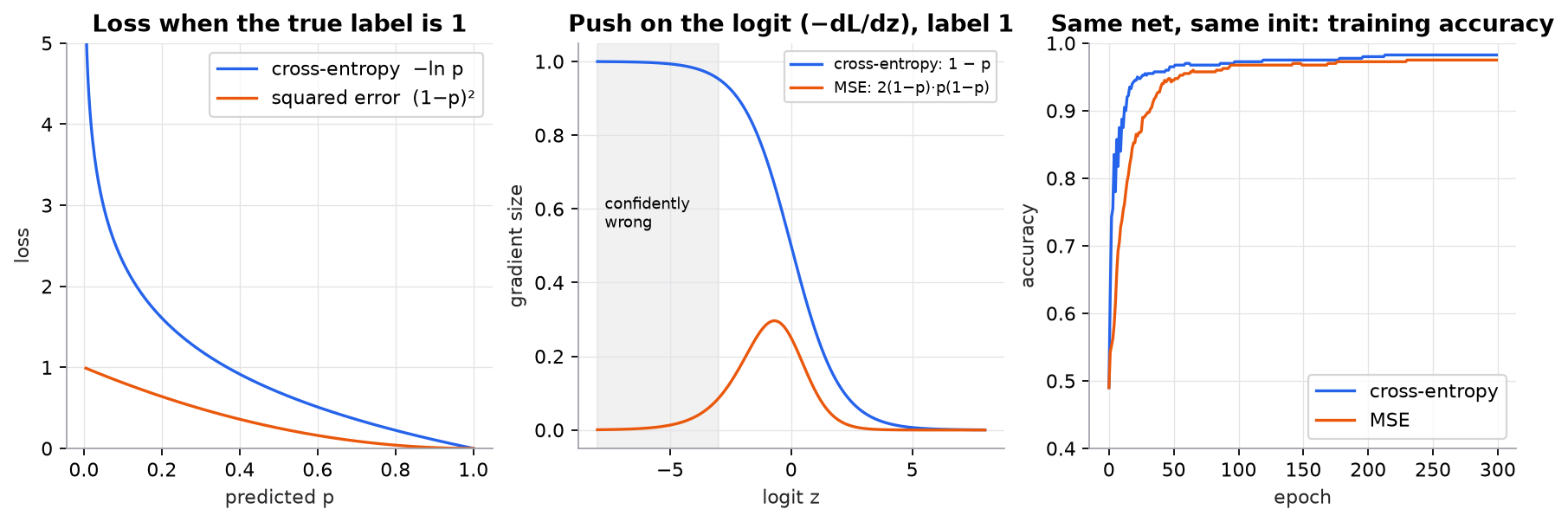
Synthetic data: 400 points uniform in a square, labelled 1 inside a circle. The network starts deliberately overconfident (large output weights), so many points begin confidently wrong. The middle panel is the reason for the right panel.
Try it (predict, then run the script):
- In the middle panel, read off the push at for both losses. The script prints them; how many times bigger is cross-entropy's?
- In the left panel, at what does cross-entropy first exceed 1? (Solve .)
- Remove the line
W2[:] *= 2.0intrainso the network starts less confident. Predict whether the gap between the curves shrinks or grows. - In the regression example, change the outlier's prediction from 16 to 106. Predict how much MSE, MAE, and Huber each grow.
3. The math
Symbols
| Symbol | Meaning | Shape |
|---|---|---|
| true target (number, 0/1 label, or class index) | scalar per example | |
| regression prediction | scalar per example | |
| logit (pre-activation output) | scalar, or for classes | |
| predicted probability of class 1 | scalar | |
| predicted class distribution | ||
| batch size | integer | |
| Huber threshold | scalar | |
| label-smoothing amount | scalar in | |
| focal-loss focusing exponent | scalar | |
| temperature (contrastive loss) | scalar |
The losses
Regression, averaged over examples with residual :
MSE is the right loss when noise is Gaussian (it is the negative log-likelihood); its minimizer is the conditional mean. MAE's minimizer is the median, which is why it ignores outliers.
Binary cross-entropy (BCE) and softmax cross-entropy:
The gradient that explains everything
With and , the chain rule gives:
The cancels for BCE and stays for MSE. When the model is confidently wrong, , so MSE's push nearly vanishes. Softmax cross-entropy has the same clean form: .
Worked example 1: confidently wrong, label 1, logit
.
- BCE gradient: .
- MSE gradient: .
Cross-entropy pushes times harder. At () the ratio is only 2 ( vs ).
Worked example 2: softmax cross-entropy and its gradient
Logits , true class 0. Softmax (from the information theory lesson) is . Loss .
Gradient . The true class's logit goes up; the others go down, each in proportion to how much probability it stole. The components sum to 0.
With label smoothing , the target becomes . Log-probabilities are , so
The loss can now never reach 0, so the model has no reason to drive logits to infinity.
Worked example 3: one outlier in regression
Targets , predictions , residuals .
- MSE: . The outlier is 99.5% of it.
- MAE: .
- Huber, : small residuals give each; the outlier gives . Total .
Worked example 4: focal loss
, with the probability of the true class. With :
| CE | weight | focal | |
|---|---|---|---|
| 0.9 (easy) | 0.1054 | 0.01 | 0.0011 |
| 0.5 | 0.6931 | 0.25 | 0.1733 |
| 0.1 (hard) | 2.3026 | 0.81 | 1.8651 |
Easy examples are discounted 100 times; hard ones keep most of their loss. In detection, where most candidate boxes are easy background, this keeps the easy majority from drowning out the rare hard cases.
Contrastive loss (InfoNCE)
For embedding models with no class labels: an anchor , one positive (an augmented view, a matching caption), and negatives :
It is softmax cross-entropy where the "correct class" is the positive. Lower sharpens the softmax. With 7 negatives, a model that can't tell them apart scores ; the script's well-separated synthetic example scores 0.125 at . Triplet loss, , is the older margin-based cousin.
4. Implementation
Build it from scratch
Regression losses are one line each. Huber uses np.where to switch from quadratic to linear at .
def mse(pred, y):
    return np.mean((pred - y) ** 2)

def mae(pred, y):
    return np.mean(np.abs(pred - y))

def huber(pred, y, delta=1.0):
    r = np.abs(pred - y)
    return np.mean(np.where(r <= delta, 0.5 * r**2, delta * (r - 0.5 * delta)))   # quadratic near 0, linear far out
Predict: at , do the two Huber pieces give the same value? (Both give , so the loss is continuous, and so is its slope.)
BCE should be computed from the logit, not from , so that log never sees 0 (see numerical stability). The gradient function is where the two classification losses differ by exactly one factor.
def sigmoid(z):
    return 1 / (1 + np.exp(-z))

def bce_with_logits(z, y):
    # -[y log s(z) + (1-y) log(1-s(z))], rewritten so exp only sees non-positive numbers
    return np.mean(np.maximum(z, 0) - z * y + np.log1p(np.exp(-np.abs(z))))

def grad_wrt_logit(z, y, loss):
    """dLoss/dz for one example with a sigmoid output p = s(z)."""
    p = sigmoid(z)
    if loss == "bce":
        return p - y                              # the sigmoid's slope cancels out
    return 2 * (p - y) * p * (1 - p)              # MSE on p: chain rule leaves p(1-p) in
Predict: for label 0 and (confidently wrong the other way), what are the two gradients?
Softmax cross-entropy works in log space, supports label smoothing by building a soft target, and has the gradient. The script checks that gradient with finite differences.
def log_softmax(z):
    z = z - z.max(axis=-1, keepdims=True)
    return z - np.log(np.exp(z).sum(axis=-1, keepdims=True))

def cross_entropy(logits, target, smoothing=0.0):
    """Mean CE over a batch. logits [n, K], target [n] ints. smoothing spreads eps over all K classes."""
    n, k = logits.shape
    q = np.full((n, k), smoothing / k)
    q[np.arange(n), target] += 1 - smoothing
    return -(q * log_softmax(logits)).sum(axis=1).mean()

def ce_grad(logits, target):
    """dCE/dlogits for one example = softmax(z) - onehot(y)."""
    g = np.exp(log_softmax(logits))
    g[target] -= 1
    return g
Predict: why do the components of ce_grad always sum to 0? (Softmax sums to 1 and you subtract exactly 1.)
Focal loss reweights cross-entropy; InfoNCE is cross-entropy over similarity scores, with the positive at index 0.
def focal_loss(p_true, gamma=2.0, alpha=1.0):
    return -alpha * (1 - p_true) ** gamma * np.log(p_true)       # (1-p)^gamma down-weights easy examples

def info_nce(anchor, positive, negatives, tau=0.1):
    """Cross-entropy where the 'correct class' is the positive among [positive, *negatives]."""
    cands = np.vstack([positive, negatives])
    sims = cands @ anchor / (np.linalg.norm(cands, axis=1) * np.linalg.norm(anchor))   # cosine similarity
    return -log_softmax(sims / tau)[0]
Predict: what does focal loss reduce to when ?
The training comparison uses one small ReLU network, trained full-batch. The only line that changes between runs is the gradient at the logit.
def train(X, y, loss, epochs=300, lr=0.5, hidden=16, seed=1):
    rng = np.random.default_rng(seed)
    W1, b1 = rng.normal(0, 1, (2, hidden)), np.zeros(hidden)
    W2, b2 = rng.normal(0, 1, hidden), 0.0
    W2[:] *= 2.0                                                   # a deliberately overconfident start
    acc = []
    for _ in range(epochs):
        H = np.maximum(X @ W1 + b1, 0)                             # [n, hidden]
        z = H @ W2 + b2                                            # [n]
        dz = grad_wrt_logit(z, y, loss) / len(y)                   # the only line that differs
        dH = np.outer(dz, W2) * (H > 0)
        W2 -= lr * H.T @ dz
        b2 -= lr * dz.sum()
        W1 -= lr * X.T @ dH
        b1 -= lr * dH.sum(axis=0)
        acc.append(((z > 0) == (y > 0.5)).mean())
    return acc
Predict: if you raised MSE's learning rate to make up for its smaller gradients, would that fix the confidently-wrong examples? (No: it scales every gradient equally, including the ones that were already fine, and can destabilize them.)
Use the library
import torch.nn.functional as F
F.mse_loss(pred, y);  F.l1_loss(pred, y);  F.huber_loss(pred, y, delta=1.0)
F.binary_cross_entropy_with_logits(z, y, pos_weight=torch.tensor([9.0]))   # takes LOGITS; pos_weight for imbalance
F.cross_entropy(logits, target, label_smoothing=0.1, weight=class_w)       # logits [n, K], target [n] int64
torchvision.ops.sigmoid_focal_loss(z, y, alpha=0.25, gamma=2.0)            # focal loss for detection
F.cross_entropy fuses log-softmax and NLL, which the scratch version made explicit. Multi-label problems (several classes can be true at once) use binary_cross_entropy_with_logits with one logit per class, not softmax. For contrastive learning, InfoNCE is usually written as F.cross_entropy(sim / tau, torch.arange(n)) over a batch similarity matrix, where the diagonal holds the positives.
Run it
uv run code/10-neural-networks/loss_functions.pyKey output:
MSE = 25.1250   MAE = 2.7500   Huber(delta=1) = 2.4375
z=-5  p=0.0067  dBCE/dz=-0.9933  dMSE/dz=-0.0132
grad = softmax - onehot = [-0.341   0.2424  0.0986]
finite-difference check max error = 7.7e-11
label smoothing eps=0.1: CE = 0.5137
p_true=0.9: CE=0.1054  focal=0.0011  weight (1-p)^2=0.01
tau=0.1: loss=0.1255
mse: accuracy at epoch 10=0.728, 50=0.945, 300=0.975
bce: accuracy at epoch 10=0.840, 50=0.965, 300=0.983
5. Engineering
Choosing a loss.
| Task | Output layer | Loss |
|---|---|---|
| Regression, Gaussian-ish noise | linear | MSE |
| Regression with outliers | linear | Huber (or MAE) |
| Binary classification | 1 logit | BCE with logits |
| Multi-class, one label per example | logits | softmax cross-entropy |
| Multi-label (tags) | logits | BCE with logits per class |
| Heavy class imbalance | as above | class weights or pos_weight; focal loss for detection |
| Overconfident classifier | logits | cross-entropy + label smoothing (around 0.1) |
| Embeddings / retrieval | normalized vectors | InfoNCE with in-batch negatives |
| Next-token prediction (LLMs) | vocab logits | softmax cross-entropy per token |
Loss vs metric. Optimize a differentiable loss; select models and thresholds on the metric. A model's validation loss can rise (it got more confident on its mistakes) while accuracy still improves. Track both.
Imbalance. With 1% positives, an unweighted loss is dominated by negatives. Reweighting (pos_weight = negatives/positives) or resampling changes the optimal predicted probabilities, so recalibrate before reading them as probabilities. Often it's better to keep the plain loss and move the decision threshold.
Contrastive training at scale. InfoNCE quality depends on the number and hardness of negatives, so batch size and temperature matter. Collapse (all embeddings identical) shows up as falling embedding variance; watch it.
Reductions and masking. reduction="mean" over a padded sequence batch averages over padding unless you mask it (ignore_index=-100 in F.cross_entropy). Mean versus sum also changes the effective learning rate.
Watch outFailure modes. Applying softmax before
F.cross_entropy(double softmax: it trains, but gradients are squashed); using softmax for multi-label data; MSE on sigmoid outputs for classification; averaging the loss over padding tokens; reporting loss to stakeholders instead of a metric they understand.
Common mistakes
- Treating "lower loss" as "better model" across different losses. A Huber loss of 2.4 and an MSE of 25 are not comparable.
- Thinking label smoothing is free. It improves calibration of the argmax class but blurs the remaining probabilities, which can hurt distillation from that model.
- Forgetting that MSE predicts the mean. If you want the median or a quantile (delivery-time promises), use MAE or a quantile loss.
6. Knowledge check
Quiz: Loss functions
What does a loss function represent in neural-network training?
Practice exercise. A binary classifier outputs logit for an example whose label is 0. Compute the BCE loss and the gradient at the logit for BCE and for MSE on .
Solution
.
BCE .
BCE gradient: . MSE gradient: . Cross-entropy pushes about 11 times harder.
Implementation challenge. Add a quantile (pinball) loss, with , to the script. Fit a single constant to the synthetic targets [1, 2, 3, 4, 100] by gradient descent for and , and compare with MSE's constant.
Solution
def pinball(pred, y, tau):
    r = y - pred
    return np.mean(np.maximum(tau * r, (tau - 1) * r))

y = np.array([1, 2, 3, 4, 100.0])
for tau in (0.5, 0.9):
    c = 0.0
    for _ in range(50000):
        g = -np.mean(np.where(y > c, tau, tau - 1))   # subgradient w.r.t. c
        c -= 0.05 * g
print(tau, round(c, 2))settles at 3 (the median). climbs all the way to 100: with only five points, the 90th percentile is the largest one, since any lower value leaves 20% of the points above it. MSE's constant is the mean, 22. Pinball loss is how you train a model to predict "90% of deliveries arrive by" instead of an average.
Summary
- The loss is what the optimizer sees; the metric is what you report. They differ.
- MSE targets the mean and punishes outliers; MAE targets the median; Huber blends them.
- Cross-entropy with a sigmoid or softmax has gradient ; MSE on probabilities keeps an extra that vanishes when the model is confidently wrong.
- Label smoothing caps confidence; focal loss down-weights easy examples; class weights handle imbalance.
- InfoNCE is cross-entropy over similarities, the workhorse of embedding training.
Next: Intro to PyTorch
Related: Information theory · Numerical stability · Logistic regression · Backpropagation
Parts of this lesson are adapted from AI Engineering from Scratch by Rohit Ghumare (MIT license, notice): Loss Functions.
Interview angle
Why use cross-entropy instead of MSE for classification?
Look at the gradient with respect to the logit. With a sigmoid output p, cross-entropy's gradient is p − y: the sigmoid's slope p(1 − p) cancels against the derivative of the log. MSE on p gives 2(p − y)·p(1 − p), so that slope stays in. When the model is confidently wrong, say logit −5 for a positive example, p is 0.0067 and p(1 − p) is tiny: cross-entropy pushes with −0.99, MSE with −0.013, about 75 times weaker. So MSE learns slowly exactly on the examples that matter most. There are two more reasons. Cross-entropy is the negative log-likelihood of a Bernoulli or categorical model, so it's the principled choice and gives calibrated probabilities. And as a function of the logits it's convex for a linear model, while MSE through a sigmoid is not. Both losses agree on the best constant prediction for uninformative data; the difference is in how hard they correct.
MSE, MAE, or Huber for a regression target with occasional huge outliers?
It depends on whether the outliers are errors or the thing you care about. MSE estimates the conditional mean and charges the square of each error, so one point off by 10 contributes 100 while points off by 0.5 contribute 0.25: in a four-point example the outlier is 99.5% of the loss and drags the fit toward itself. MAE estimates the median and charges linearly, so it's robust, but its gradient has constant size near zero, which can make convergence jittery. Huber is quadratic below a threshold delta and linear above, so it behaves like MSE on normal points and like MAE on outliers; it's my default when outliers are noise, with delta set around the typical residual scale. If the outliers are real and costly, like rare huge orders, I keep MSE or model them explicitly. If the business needs a guarantee, I use a quantile loss instead.
Your multi-class classifier trains, but accuracy plateaus well below a baseline and predicted probabilities are all close to uniform. You find `loss = F.cross_entropy(F.softmax(logits, -1), y)`. What's wrong?
That's a double softmax. F.cross_entropy expects raw logits and applies log-softmax itself, so here the probabilities from softmax are being treated as logits. They're all between 0 and 1, so the second softmax sees inputs that differ by at most 1, and its output can never be far from uniform: with 10 classes the true class can get at most about e/(e + 9), roughly 0.23. The loss can't go below about 1.46, and the gradients are squashed by the extra softmax's Jacobian, so training stalls. The fix is to pass logits directly. The same family of bugs: sigmoid before binary_cross_entropy_with_logits, or applying softmax for a multi-label problem where you need independent sigmoids. A quick check is the step-0 loss: it should be about ln K. Also check that the model's last layer has no activation.
You're training a fraud classifier with 0.5% positives. How do you set up the loss?
Start with plain BCE with logits and a stratified validation set, and measure precision-recall AUC and recall at the precision the business needs, not accuracy, since predicting "never fraud" scores 99.5%. If the model under-learns positives, add pos_weight around negatives/positives, here about 199, or a milder value like the square root, about 14, and tune it on validation. Weighting shifts the predicted probabilities upward, so recalibrate (Platt scaling or isotonic regression) before anyone reads them as probabilities. Focal loss is an option if there are many easy negatives that dominate the gradient; it's standard in object detection with gamma 2. Often the cleanest approach is no reweighting at all: train the calibrated model and move the decision threshold to hit the precision target. Whatever I pick, I'd compare the variants on the same validation metric and check calibration curves.