Module 21: Safety and security 45 min14 min quick readAI engineering
Differential privacy
Define (ε, δ)-differential privacy, apply the Laplace and Gaussian mechanisms, train with DP-SGD (per-example clipping plus noise) and track the privacy budget, and decide when DP is the right defense against memorization in ML and LLM systems.
Before this: Probability and statistics, Gradient descent
Quick read: the intuition, interactive visualization, summary, and interview questions. The math, implementation, engineering, and knowledge-check sections are hidden.
Mental model. Differential privacy is a promise about plausible deniability. Whatever the system outputs, it would have been almost as likely to output the same thing if your record had never been in the data. So nobody looking at the output, however clever and whatever else they know, can tell much about you. The price is noise: the stronger the promise, the blurrier the answer.
You will learn to
- State the definition of (ε, δ)-differential privacy and read what ε and δ mean in practice.
- Apply the Laplace mechanism to a count and the Gaussian mechanism to a sum, using sensitivity to set the noise.
- Explain DP-SGD: per-example gradient clipping, Gaussian noise, and a privacy accountant that adds up the budget over steps.
- Compute ε for a training run and explain why more data makes privacy cheaper.
- Distinguish what DP protects against (membership inference, memorization of individual records) from what it does not (secrets repeated across many records, prompt-time leaks).
- Choose between DP training, DP fine-tuning with LoRA, and non-DP controls for an LLM product.
Why it matters. Models memorize. Large language models have been shown to reproduce verbatim training text, including personal details, when prompted the right way (Carlini et al. 2021). If you train or fine-tune on user data (support tickets, medical notes, keyboard input), "we removed the names" is not a guarantee. Differential privacy is the one defense with a mathematical bound, and it is used in production by the US Census Bureau, by Apple and Google for device telemetry, and for private model training.
1. Intuition
Neighbouring datasets. Take a dataset and make by adding or removing one person's record. A mechanism (a query, a training run) is private if its outputs on and are hard to tell apart. If they are, the output cannot reveal much about that person, because it would have looked about the same without them.
ε is the privacy budget. ε bounds how much more likely any output is with your record than without it: at most times. With ε = 0.5, that factor is 1.65; with ε = 1, it is 2.7; with ε = 10, it is 22,000, which is barely a promise. δ is a small probability that the bound fails, set far below one over the dataset size (for example for 10,000 people).
Noise sized to sensitivity. The sensitivity of a query is the most one record can change its answer. A count has sensitivity 1: one person changes it by at most 1. To hide that change, add random noise a few times larger than the sensitivity. Larger noise, smaller ε, stronger privacy, less accurate answer.
Composition: privacy is spent, not kept. Every query or training step that touches the data spends some budget, and the costs add up. Answer the same question 100 times with fresh noise and someone can average the noise away. A privacy accountant tracks the total ε across everything you release.
Post-processing is free. Anything computed from a DP output, without touching the data again, is just as private. Train a model with DP and you can share its weights, its predictions, and its generated text without spending more budget.
DP-SGD: privacy for training. Training is many steps, each a sum of per-example gradients. DP-SGD (Abadi et al. 2016) makes each step a Gaussian mechanism:
- Compute the gradient of each example separately.
- Clip each to a maximum L2 norm . Now no single example can move the sum by more than : the sensitivity is .
- Sum the clipped gradients and add Gaussian noise with standard deviation .
- Take the step. The accountant adds this step's cost to the total.
Usually each step uses a random mini-batch. Sampling helps: an example that is in a given batch only with probability is better hidden, which amplifies privacy and lowers ε a lot.
Why more data helps. The noise is added to the sum of gradients, and its size depends on and , not on the batch. Divide by the batch size to get the average gradient, and the noise per example shrinks. With many examples, the signal (the true gradient) dominates; with few, the noise does. DP works best when there are many people and you want patterns, not individuals.
Key distinctionDP protects individuals, not secrets. If a fact appears in many records (an API key pasted in a thousand tickets, a fact everyone knows), DP may let the model learn it, because no single record is responsible. DP bounds what the output reveals about any one record. Scrub secrets separately.
2. Visualization
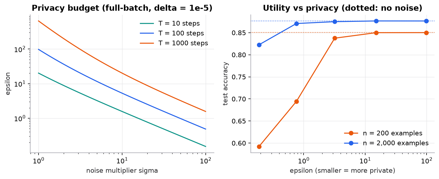
Synthetic data. Left: ε falls as noise rises and grows with the number of steps (composition). Right: the same privacy budget costs far less accuracy with ten times more data.
Try it (run differential_privacy.py, predict first, then check):
- Release the patient count 100 times at ε = 0.5 each and average. Predict how close the average is to 100, then compute the total ε by simple addition.
- Change the clip norm from 1.0 to 0.1 with σ fixed. Predict whether ε changes, and whether accuracy changes.
- Double the number of steps to 200 at σ = 16. Predict ε before running.
- In
make_data, multiply the signal by 3 (X @ (3 * TRUE_W)). Predict whether the small-data model still collapses at ε = 0.76.
3. The math
Symbols
| Symbol | Meaning | Shape / unit |
|---|---|---|
| randomized mechanism (query or training run) | ||
| neighbouring datasets (differ in one record) | ||
| privacy loss bound | ≥ 0 | |
| failure probability | small, e.g. | |
| sensitivity: max change in the output from one record | output units | |
| Laplace noise scale | output units | |
| per-example gradient | ||
| clipping norm | ≥ 0 | |
| noise multiplier (noise std is ) | ≥ 0 | |
| , | training steps; Rényi order | count; |
Definition
is -differentially private if for all neighbouring and every set of outputs :
Laplace mechanism
Release with . This is -DP.
Worked example. A clinic releases how many patients have condition X. The true count is 100; the neighbour has 101. , .
- Noise scale: .
- Probability the release lands in when the truth is 100: the noise must be within , so .
- Same interval when the truth is 101: the noise must be between and , so .
- Ratio: . ✓ The bound holds with room to spare for this set; it is tight for sets far out in one tail.
- Typical error: the mean absolute value of Laplace noise is patients.
Gaussian mechanism and Rényi accounting
Adding to a query with L2 sensitivity satisfies Rényi DP of order with cost . Rényi costs add across steps, and convert to by minimizing over :
This is exact for full-batch DP gradient descent: every step uses every example, so steps are Gaussian mechanisms with sensitivity .
Worked example. steps, , .
- First term at order : .
- Second term: , so .
- Minimum where the derivative is zero: , so , , .
- .
- That is a weak guarantee. Quadrupling noise to gives ; mini-batch sampling with probability would lower it much further, which is why real DP-SGD samples batches.
DP-SGD step
The noise in has standard deviation per coordinate. At , : with it is ; with it is , ten times smaller, while each clipped gradient stays at most 1. That is the right panel of the figure.
4. Implementation
Build it from scratch
The full script is code/21-safety-security/differential_privacy.py. NumPy only; all data is synthetic. The training loop is full-batch DP gradient descent so that the simple accountant is exact.
The Laplace mechanism is one line. Noise scale is sensitivity over ε.
def laplace_count(true_count, epsilon, sensitivity=1.0):
    return true_count + rng.laplace(0.0, sensitivity / epsilon)
Predict: you release the count of a group with 3 people at ε = 0.5. Roughly how useful is the answer?
The accountant. Rényi cost per Gaussian step is ; costs add over steps; then search over orders for the smallest .
def epsilon(sigma, steps, delta):
    """RDP of one Gaussian mechanism at order a is a / (2 sigma^2); T steps add; convert with log(1/delta)/(a-1)."""
    eps = steps * ALPHAS / (2 * sigma**2) + math.log(1 / delta) / (ALPHAS - 1)
    i = int(np.argmin(eps))
    return float(eps[i]), float(ALPHAS[i])
Predict: doubling the steps at fixed σ multiplies ε by roughly what factor (hint: the best order also moves)?
DP gradient descent. Per-example gradients, clip each row, add noise to the sum, step. These four lines are the whole idea of DP-SGD.
def dp_gd(X, y, sigma, clip, steps, lr=0.5):
    n, w = len(y), np.zeros(X.shape[1] + 1)
    Xb = np.hstack([X, np.ones((n, 1))])                         # [n, 21]: 20 features + a bias column
    for _ in range(steps):
        p = 1 / (1 + np.exp(-Xb @ w))
        g = (p - y)[:, None] * Xb                                # per-example gradients, [n, 21]
        norms = np.linalg.norm(g, axis=1, keepdims=True)
        g = g / np.maximum(1.0, norms / clip)                    # clip each row to L2 norm <= clip
        noisy_sum = g.sum(0) + rng.normal(0, sigma * clip, size=w.shape)  # sensitivity of the sum is `clip`
        w -= lr * noisy_sum / n
    return w
Predict: what goes wrong with the privacy guarantee if you clip the batch gradient instead of each example's gradient?
Use the library
Opacus adds DP-SGD to a PyTorch training loop. It computes per-example gradients efficiently, clips, adds noise, samples batches with Poisson sampling, and runs an accountant that includes the subsampling amplification:
from opacus import PrivacyEngine

engine = PrivacyEngine(accountant="rdp")
model, optimizer, loader = engine.make_private_with_epsilon(
    module=model, optimizer=optimizer, data_loader=loader,
    target_epsilon=3.0, target_delta=1e-5, epochs=5, max_grad_norm=1.0)  # picks sigma for the target
# ...train as usual...
print(engine.get_epsilon(delta=1e-5))
TensorFlow Privacy and JAX libraries offer the same. For LLMs, the common recipe is DP fine-tuning of a small adapter: freeze the base model, train LoRA weights with DP-SGD. Fewer trainable parameters means less memory for per-example gradients and less total noise. The guarantee then covers the fine-tuning data, not whatever the base model memorized in pretraining. Google's open-source DP libraries and OpenDP cover DP statistics (counts, sums, histograms).
Run it
uv run code/21-safety-security/differential_privacy.pyKey lines of output:
P(output in [99.5, 100.5] | count=100) = 0.2212;  | count=101) = 0.1532;  ratio 1.444 <= e^eps = 1.649
sigma=4: best order a=2.92: 100*2.92/(2*16) + ln(1e5)/(2.92-1) = 15.12
n=  200  sigma=64.0  epsilon=   0.76  test accuracy=0.694 (mean of 5 runs)
n=  200  sigma=256.0  epsilon=   0.19  test accuracy=0.592 (mean of 5 runs)
n= 2000  sigma=64.0  epsilon=   0.76  test accuracy=0.871 (mean of 5 runs)
n= 2000  sigma=256.0  epsilon=   0.19  test accuracy=0.823 (mean of 5 runs)
5. Engineering
Define the unit of privacy. DP protects "one record". Decide whether that is one example, one document, or one user. If a user contributes 500 support tickets, example-level DP with ε = 2 can leak much more about that user. User-level DP (clip each user's total contribution) is what most products actually need.
Pick ε and report it honestly. There is no universal safe value. Single-digit ε with δ well below is a common target for training; ε near 1 or below is strong. Always report ε together with δ, the unit of privacy, the accountant, and whether batch sampling was really random as the accountant assumed.
Hyperparameters spend budget too. Every training run on private data spends ε. Tuning 20 configurations and keeping the best leaks more than one run. Tune on public or synthetic proxies, or account for the search.
Cost. Per-example gradients take more memory and time than a normal backward pass; DP fine-tuning usually needs larger batches and more epochs to reach good accuracy. The accuracy cost falls as the dataset grows (the figure), and is worst for rare classes and small subgroups, which interacts with fairness: DP can hurt minority groups more because their signal is smallest.
Audit empirically. A bug in clipping or sampling silently voids the guarantee. Check with membership inference (can an attacker tell whether a record was trained on, from the model's loss?) and canaries (insert unique fake secrets and see whether the model completes them). These give lower bounds on leakage; DP gives the upper bound.
Alternatives and complements for LLM products. If DP training is too costly: scrub PII and secrets before training, deduplicate (repeated text is memorized far more), filter outputs for training-data regurgitation, and limit what the API exposes (raw log-probabilities help attackers). For data that only appears in prompts or retrieval at inference time, DP training does nothing: protect it with access control, as in Securing AI systems. DP synthetic data is another route: train a generator with DP, then share or train on its samples.
Watch outFailure modes. Clipping the batch gradient instead of per-example gradients; shuffled fixed batches accounted as if Poisson-sampled; ε reported per epoch instead of in total; example-level DP for data where one user has many records; ignoring the budget spent on tuning; and assuming DP training protects secrets that appear in many records or in prompts.
Common mistakes
- Thinking "anonymized" (names removed) data is private. Linkage with other data re-identifies people.
- Quoting ε without δ, the unit of privacy, or the accountant.
- Adding noise to the final model weights once instead of during training; the sensitivity of trained weights is unbounded without clipping.
- Expecting DP to stop the model from learning common facts. It is not supposed to.
- Applying DP to a tiny dataset and concluding "DP doesn't work" when the problem is the data size.
- Forgetting post-processing is free, and adding noise twice.
6. Knowledge check
Quiz: Differential privacy
What does (ε, δ)-differential privacy guarantee?
Practice exercise. A survey releases the average age (ages clipped to 0 to 100) of 1,000 respondents with the Laplace mechanism at ε = 0.5. What is the sensitivity of the average, the noise scale, and the expected absolute error? How does the error change for 100 respondents?
Solution
Changing one respondent moves the sum by at most 100, so the average by at most years. (Treating as public.) Noise scale years, and the expected absolute error of Laplace noise is years.
With 100 respondents: sensitivity , years, ten times worse. Same privacy, ten times less data, ten times more error.
Implementation challenge. Add Poisson batch sampling to dp_gd: each step, include each example independently with probability , clip and noise the batch sum, and divide by the expected batch size . Compare accuracy with full-batch training at the same σ and 10 times as many steps.
Solution sketch
Each step: mask = rng.random(n) < q, compute and clip gradients for X[mask], add N(0, σ²C²) noise to their sum, divide by q * n. Dividing by the expected size (not the realized one) keeps the sensitivity fixed at . Ten times as many steps gives each example the same expected number of updates. Accuracy should be similar or better. The privacy cost is lower than the full-batch formula suggests because of amplification by subsampling, but computing it needs the subsampled-Gaussian accountant, which is what Opacus implements; the simple formula in this script would overstate ε.
Summary
- (ε, δ)-DP bounds how much any output can depend on one record: probabilities change by at most a factor , except with probability δ.
- Noise is sized to sensitivity: Laplace with for counts, Gaussian for sums of clipped vectors.
- Costs compose over queries and steps; an accountant tracks the total, and post-processing is free.
- DP-SGD clips each example's gradient to , adds to the sum, and accounts every step; batch sampling amplifies privacy, and more data makes the noise relatively smaller.
- DP protects individual records, not facts repeated across many records or data supplied at inference time; pair it with scrubbing, deduplication, and access control.
Next: ML system design
Related: Securing AI systems · Fairness · Fine-tuning in practice · Gradient descent
Parts of this lesson are adapted from AI Engineering from Scratch by Rohit Ghumare (MIT license, notice): Differential Privacy for LLMs.
Interview angle
Explain differential privacy and what epsilon actually means.
A mechanism is differentially private if its output distribution barely changes when you add or remove one person's record. Formally, the probability of any output with your record is at most e to the epsilon times the probability without it, plus a small delta. So epsilon bounds how much an observer, whatever else they know, can learn about whether you were in the data. Epsilon 0.5 means probabilities can shift by at most a factor of about 1.65; epsilon 10 allows a factor of 22,000, which is a weak guarantee. Delta is the small chance the bound fails, set well below one over the number of people. Two properties make it practical: costs add up across queries and training steps, so you track a total budget; and anything computed from a private output is equally private, so a DP-trained model can be shared freely.
Walk me through DP-SGD. Why clip per example, and why does more data help?
At each step, compute each example's gradient separately, clip each one to a maximum norm C, sum them, add Gaussian noise with standard deviation sigma times C, then divide by the batch size and update. Clipping per example is what bounds the sensitivity: no single example can move the sum by more than C, so noise proportional to C hides any one person. If you clipped the batch gradient instead, one outlier example could still dominate it and the guarantee would be gone. An accountant adds up each step's privacy cost, with batch sampling lowering it. More data helps because the noise is added to the sum, so its size doesn't grow with the batch, while the signal does. After dividing by n, the noise per example shrinks like one over n. Small datasets pay a big accuracy cost; large ones barely notice.
Your team fine-tuned an LLM on support tickets with DP at epsilon 3, but it still outputs a customer's API key when prompted. How is that possible?
A few possibilities. The unit of privacy may be wrong: if the guarantee is per example, and that customer pasted the key into fifty tickets, the key is spread across fifty records and the per-example bound says little about it. If many customers shared the same leaked key, it's a common fact rather than an individual record, and DP allows learning it. The key may have come from somewhere else: the base model's pretraining data, or a retrieval system or prompt context at inference time, which DP training doesn't cover. Or the implementation is broken: batch clipping instead of per-example clipping, or accounting that assumed random sampling the data loader didn't do. I'd check where the key appears in the training data, verify the clipping and sampling code, move to user-level DP, and scrub secrets before training regardless.
Full-batch DP gradient descent runs for 100 steps with noise multiplier 4 and delta 1e-5. Roughly what epsilon do you get, and how would you lower it?
With the Rényi accountant, each Gaussian step costs alpha over two sigma squared, so 100 steps cost 100 alpha over 32, about 3.1 alpha. Converting to epsilon adds ln of one over delta, about 11.5, divided by alpha minus one. Minimizing over alpha gives alpha near 2.9 and epsilon about 9.1 plus 6.0, roughly 15. That's a weak guarantee. Levers: more noise, since sigma 16 gives about 3.2; fewer steps, since epsilon grows with the number of steps; and, most effective in practice, random mini-batches instead of full batches, because if each example is used in a step only with probability q, privacy is amplified and epsilon drops a lot. More data doesn't lower epsilon directly, but it lets you afford more noise at the same accuracy.