The Python toolkit

1. Intuition

A NumPy array is a block of numbers of a single type with a shape. Operations apply element by element across the whole block, implemented in C. "Standardize every column" is one line: subtract the column means, divide by the column standard deviations.

Broadcasting lets arrays of different shapes combine: a [1000, 3] matrix minus a [3] vector subtracts the vector from every row. NumPy lines up shapes from the right and stretches dimensions of size 1.

pandas adds column names, mixed types, missing-value handling, and group-by on top of NumPy. Use it to explore and clean; convert to NumPy arrays (or pass DataFrames to scikit-learn) for modeling.

2. Visualization

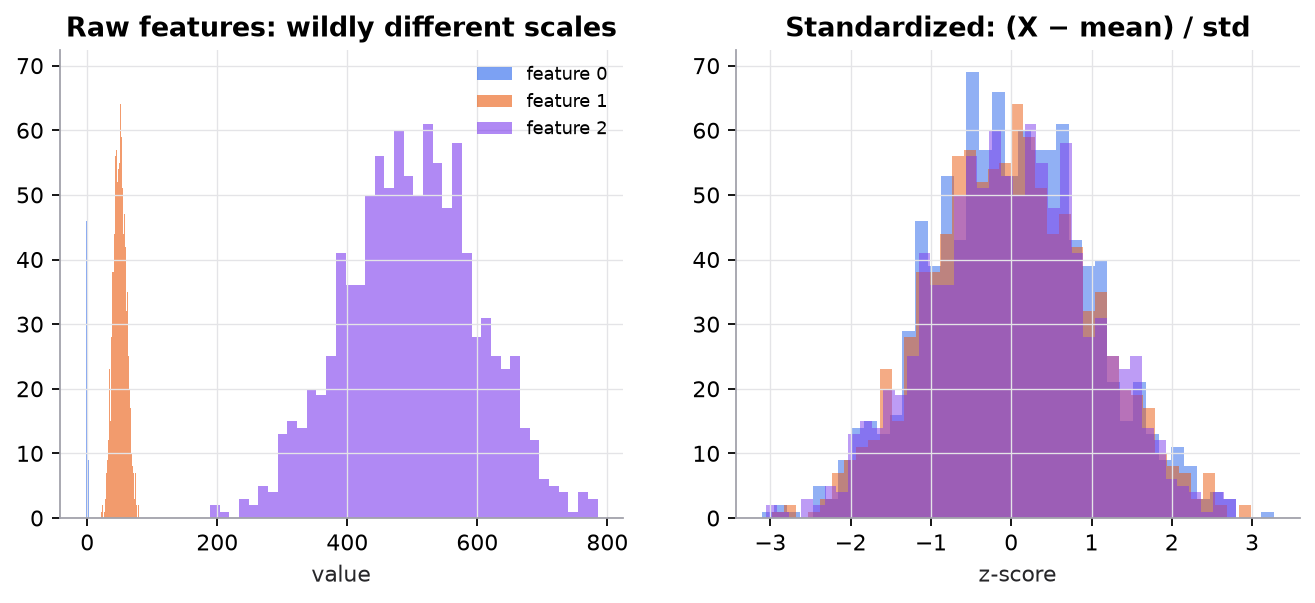
One broadcasting line, (X - X.mean(axis=0)) / X.std(axis=0), standardizes all three columns.

3. The math

Broadcasting rules

Compare shapes from the rightmost dimension:

1. Dimensions are compatible if they are equal or one of them is 1.
2. Missing leading dimensions are treated as 1.
3. The result takes the larger size in each dimension.

Axis reductions

For $X$ of shape $[n, p]$: X.mean(axis=0) averages over rows, giving one value per column, shape $[p]$. X.mean(axis=1) gives one value per row, shape $[n]$.

Worked example

$X = \begin{bmatrix}1 & 10\\3 & 30\end{bmatrix}$. Column means: $[2, 20]$. Population standard deviations: $[1, 10]$. Standardized: $\frac{X - [2, 20]}{[1, 10]} = \begin{bmatrix}-1 & -1\\1 & 1\end{bmatrix}$. Each column now has mean 0 and standard deviation 1.

4. Implementation

You will rebuild the two ideas that make NumPy fast and occasionally surprising: an array is a flat buffer plus a shape and strides, and broadcasting follows a three-rule shape check. Then the everyday NumPy, pandas, and matplotlib code you will write in every later lesson.

Build it from scratch

Every n-dimensional array is stored as one flat run of numbers. Strides say how many elements to skip to move one step along each axis. In row-major (C) order the last axis is contiguous, so its stride is 1, and each earlier stride is the product of the sizes after it.

def strides_for(shape):
    """Row-major (C order): the last axis moves fastest, so its stride is 1 element."""
    strides = [1] * len(shape)
    for i in range(len(shape) - 2, -1, -1):
        strides[i] = strides[i + 1] * shape[i + 1]
    return strides

def flat_index(index, strides):
    return sum(i * s for i, s in zip(index, strides))

Predict: for shape (2, 3, 4), what are the strides, and at which flat position does element [1, 2, 3] live?

This is why reshape and transpose are usually free: they write new shape and stride numbers and leave the buffer alone (a view). A transposed array is no longer contiguous, which is why some operations (.view() in PyTorch, for one) then demand a copy.

Broadcasting is section 3's rule, written out. Walk the shapes from the right; each pair must match or contain a 1, and missing dimensions count as 1.

def broadcast_shape(a, b):
    """Align shapes from the right; each pair of dims must be equal or one of them must be 1."""
    out = []
    for i in range(1, max(len(a), len(b)) + 1):
        da = a[-i] if i <= len(a) else 1
        db = b[-i] if i <= len(b) else 1
        if da != db and 1 not in (da, db):
            raise ValueError(f"cannot broadcast {a} with {b}: {da} vs {db}")
        out.append(max(da, db))
    return tuple(reversed(out))

Predict: what do (8, 1, 6) with (7, 1) and (3, 2) with (3,) give? Which line of the table in section 3 does (1000,) with (1000, 1) match, and why is it usually a bug?

Use the library

Real work uses NumPy for arrays, pandas for labelled tables, and matplotlib for plots. Seed the generator so every run gives the same numbers.

import numpy as np
import pandas as pd
import matplotlib.pyplot as plt

rng = np.random.default_rng(42)                     # seeded: same numbers every run

# NumPy: vectorized standardization
X = rng.normal(size=(1000, 3)) * [1, 10, 100] + [0, 50, 500]
Z = (X - X.mean(axis=0)) / X.std(axis=0)            # [1000,3] - [3] broadcasts per row

# pandas: load, inspect, clean, aggregate
df = pd.DataFrame({"city": rng.choice(["A", "B", "C"], 1000), "price": rng.normal(300, 50, 1000)})
df.loc[rng.choice(1000, 20, replace=False), "price"] = np.nan
print(df.describe())                                # summary statistics
print(df.isna().sum())                              # missing values per column
df["price"] = df["price"].fillna(df["price"].median())
print(df.groupby("city")["price"].agg(["mean", "count"]))

# matplotlib: always label axes
fig, ax = plt.subplots()
ax.hist(df["price"], bins=40)
ax.set(xlabel="price ($k)", ylabel="count", title="Price distribution")
fig.savefig("price.png", dpi=150)

What the library adds: compiled loops over the flat buffer (the speed), np.broadcast_shapes (the scratch function above), and arr.strides, np.shares_memory, and arr.flags to inspect views. PyTorch tensors use the same shape, stride, and broadcasting model, so this transfers directly.

Run it

From guide/:

uv run code/00-foundations/tensors_scratch.py

shape (2, 3, 4) -> strides [12, 4, 1] (elements)
element [1, 2, 3] lives at flat position 23 -> 23
NumPy strides in bytes (96, 32, 8) = [12, 4, 1] × 8 bytes
transpose is a view: shape (4, 2, 3), strides (8, 96, 32), shares memory: True
contiguous after transpose? False
broadcast (1000, 3) with (3,) -> (1000, 3)
broadcast (4, 1) with (1, 5) -> (4, 5)
broadcast (8, 1, 6) with (7, 1) -> (8, 7, 6)
cannot broadcast (3, 2) with (3,): 2 vs 3
python loop 0.118s, vectorized 0.0012s, same result: True
all checks match NumPy

The timing line varies by machine; on a laptop the vectorized version is typically around 100× faster. Full script: code/00-foundations/tensors_scratch.py. The figure comes from code/00-foundations/foundations.py. The repository pins its dependencies in pyproject.toml; uv run creates the same environment on any machine.

5. Engineering

Reproducibility. Fix random seeds (np.random.default_rng(seed), random_state= in scikit-learn), pin package versions, and record the data version. An experiment you can't rerun is an anecdote.

Performance. Vectorize; avoid df.apply with Python functions on large frames; use appropriate dtypes (float32, category). Out-of-memory data needs chunking or tools like Polars, DuckDB, or Spark.

Exploratory data analysis checklist. Shape and dtypes; missing values per column; duplicates; distributions and outliers; target balance; time ranges; obviously leaky columns (IDs, timestamps after the event, "status" fields).

Watch out

Failure modes. Accidental [n] - [n, 1] broadcasting; chained pandas indexing (df[df.a > 0]["b"] = 1) that silently modifies a copy; integer division and dtype overflow; filling missing values using statistics from the whole dataset (leakage).

Common mistakes

• Looping over rows instead of using column operations.
• Forgetting axis= and reducing the whole array to one number.
• Unseeded randomness, so results change every run.

6. Knowledge check

Practice exercise. Without running it, give the shape of A + B for A.shape == (5, 1, 4) and B.shape == (3, 1).

Implementation challenge. Load any CSV with pandas, write an EDA function that prints missing values, duplicate count, numeric summaries, and the five most common values of each categorical column, and plot a histogram of every numeric column.

Summary

• NumPy operates on whole arrays; broadcasting aligns shapes from the right.
• Reduce with an explicit axis; check shapes after every step.
• pandas handles loading, cleaning, missing values, and group-bys; plot with labeled axes.
• Seed randomness and pin versions so experiments are reproducible.

Next: Information theory

Related: The ML workflow

Go deeper, code-first (AI Engineering from Scratch): Debugging and Profiling · Python for AI Engineering

Parts of this lesson are adapted from AI Engineering from Scratch by Rohit Ghumare (MIT license, notice): Tensor Operations.

Interview angle