Module 0: Mathematical and programming foundations 40 min9 min quick readMathematics
Information theory
Compute surprise, entropy, cross-entropy, KL divergence, and perplexity by hand, and explain why the classification loss you minimize is exactly cross-entropy.
Before this: Probability and statistics, Calculus for ML
Quick read: the intuition, interactive visualization, summary, and interview questions. The math, implementation, engineering, and knowledge-check sections are hidden.
Mental model. Information is surprise. A rare event tells you a lot, a certain event tells you nothing. Entropy is the average surprise of a distribution. Cross-entropy is the average surprise you feel when reality follows one distribution but you predicted another. Training a classifier means shrinking that second number.
You will learn to
- Compute surprise and entropy in bits and nats.
- Compute cross-entropy and KL divergence, and show that cross-entropy = entropy + KL.
- Explain why minimizing cross-entropy is the same as maximizing log-likelihood.
- Convert a language model's average loss into perplexity and interpret it.
- Say what mutual information measures and when it beats correlation.
Why it matters. Every classifier and every language model in this course is trained with cross-entropy. Perplexity is reported for every language model. KL divergence appears in knowledge distillation, variational autoencoders, and RLHF (the KL penalty that keeps a tuned model close to its base). They are one idea seen from different angles. Learn it once here and the loss curves later will make sense.
1. Intuition
Suppose a friend texts you the result of a coin flip. If the coin is fair, the message settles a real question: one bit of information. If the coin lands heads 99% of the time, a "heads" text tells you almost nothing, because you already expected it. A "tails" text is a big surprise.
So surprise grows as probability falls. A certain event has zero surprise. A one-in-a-thousand event has a lot.
Entropy is the average surprise you expect from a distribution before you see the outcome. A fair coin has the highest possible entropy for two outcomes (1 bit). A 99% coin has very little (0.08 bits). Entropy is also the smallest average number of bits any code can use to send outcomes from that distribution, which is why you can't compress random noise.
Now suppose you believe the wrong distribution. Reality follows , but you bet on . Every time something happens that you thought unlikely, you are more surprised than you should be. Your average surprise under the wrong beliefs is the cross-entropy. It is always at least the entropy. The gap between the two, the extra surprise caused purely by wrong beliefs, is the KL divergence.
A classifier is a set of beliefs about labels. The true label is what reality did. The loss you minimize, , is the surprise the model felt. Averaged over the training set, that is cross-entropy. Pushing it down pushes the model's beliefs toward reality.
Perplexity turns that average surprise back into a count. A language model with perplexity 20 is as unsure, on average, as if it were picking uniformly among 20 tokens.
2. Visualization
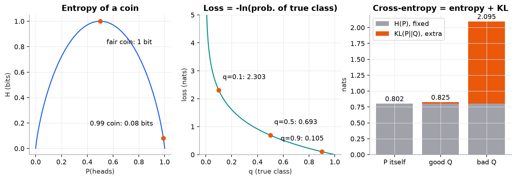
All distributions are small hand-picked examples. Left: entropy peaks when you are most unsure. Middle: the classification loss barely punishes a confident correct answer but explodes as the true class's probability goes to 0. Right: cross-entropy splits into a part the model can't change (the entropy of the data) and a part it can (KL).
Try it (predict first, then check with the script):
- In the left panel, what is the entropy of a coin with P(heads) = 0.75? Predict whether it is above or below 0.5 bits, then compute .
- In the middle panel, how much does the loss drop when a correct prediction goes from 0.9 to 0.99? Compare that with going from 0.1 to 0.2. Which change gives the bigger training signal?
- In the right panel, could any model make the bar shorter than 0.802 nats? Why not?
- Swap and the bad in
kl_divergence. Predict whether the bar height stays the same.
3. The math
Symbols
| Symbol | Meaning | Shape |
|---|---|---|
| , | true probability of outcome ; the true distribution | vector of probabilities summing to 1 |
| , | model's predicted probability; the model's distribution | same as |
| surprise (information content) of outcome | scalar | |
| entropy of | scalar | |
| cross-entropy of relative to | scalar | |
| KL divergence from to | scalar, | |
| index of the true class | integer in | |
| number of examples or tokens | integer |
Log base 2 gives bits; natural log gives nats. PyTorch, JAX, and NumPy losses use nats. bits.
Definitions
Terms with contribute 0 (the limit of ). If for an outcome that can happen, the cross-entropy is infinite: the model called it impossible.
KL is not symmetric: in general, so it is not a distance.
Cross-entropy with a one-hot label is the classification loss
With a one-hot target, and every other , so the sum keeps one term:
Over a dataset, the mean loss is . The likelihood of the data is ; its log is . So mean cross-entropy = negative log-likelihood / N. Minimizing one maximizes the other. And since of the labels doesn't depend on the model, minimizing cross-entropy also minimizes KL.
Perplexity
It is the exponential of the mean loss in nats (use if the loss is in bits). Equivalently, it is 1 over the geometric mean of the probabilities given to the true tokens.
Worked example 1: entropy, cross-entropy, KL
True distribution . Good model . All in nats.
Entropy:
Cross-entropy:
KL: (the script, with unrounded logs, prints 0.8245 and 0.0227). The bad model gives and KL : almost all of its loss is avoidable. Reversed, .
Worked example 2: one classification loss
Logits , true class 0. Softmax: subtract the max (2.0) to get , exponentiate to , sum , so .
Loss nats bits.
Worked example 3: perplexity
A model gives the true next token probabilities over four steps.
Check by geometric mean: , and . A uniform guess over 50 tokens gives loss and perplexity exactly 50.
Two extensions you will meet
Label smoothing replaces the one-hot target with . With and , the target becomes , whose entropy is 0.349 nats instead of 0. The model can no longer reach zero loss by pushing logits to infinity, which tends to improve calibration.
Mutual information measures how much knowing reduces uncertainty about :
It is 0 exactly when and are independent and catches any dependence, not just linear ones. The joint table has bits; the uniform table has 0. Decision trees pick splits by this quantity (it is information gain).
4. Implementation
Build it from scratch
Surprise and entropy first. surprise is written as so that a certain event prints 0.0 rather than −0.0. entropy skips zero-probability outcomes, which contribute nothing.
def surprise(p, base=math.e):
    """Information content of an event with probability p: -log p."""
    return math.log(1 / p) / math.log(base)   # = -log p, written so p = 1 gives +0.0

def entropy(p, base=math.e):
    """Average surprise. Terms with p = 0 contribute 0 (the limit of p log p)."""
    return sum(pi * surprise(pi, base) for pi in p if pi > 0)
Predict: what does entropy([1/6] * 6, 2) return, and why is it exactly ?
Cross-entropy scores outcomes from with the model's . The math.inf branch is the "model said impossible" case. KL is defined as the difference, so it inherits both.
def cross_entropy(p, q, base=math.e):
    """Average surprise when events come from p but you score them with q."""
    total = 0.0
    for pi, qi in zip(p, q):
        if pi > 0:
            if qi == 0:
                return math.inf          # q says "impossible" for something that happens
            total += pi * surprise(qi, base)
    return total

def kl_divergence(p, q, base=math.e):
    """Extra surprise from using q instead of p: H(p, q) - H(p). Never negative."""
    return cross_entropy(p, q, base) - entropy(p, base)
Predict: kl_divergence([1, 0], [0.5, 0.5]) versus kl_divergence([0.5, 0.5], [1, 0]). One is finite and one is infinite. Which?
Now the loss a classifier uses. Softmax turns logits into (the max subtraction is the overflow guard from numerical stability); with a one-hot target the cross-entropy is one log.
def softmax(logits):
    m = max(logits)                      # subtract the max so exp never overflows
    exps = [math.exp(z - m) for z in logits]
    s = sum(exps)
    return [e / s for e in exps]

def cross_entropy_loss(logits, target):
    """One-hot target: H(p, q) collapses to -log q[target]."""
    return -math.log(softmax(logits)[target])
Predict: if every logit is equal and there are 10 classes, what is the loss? (This is the number to check at step 0 of any training run.)
Perplexity is the exponential of the mean negative log-probability of the true tokens.
def perplexity(true_token_probs):
    """exp of the average negative log-probability of the observed tokens."""
    nll = sum(-math.log(p) for p in true_token_probs) / len(true_token_probs)
    return nll, math.exp(nll)
Predict: if one token in a long sequence gets probability , does perplexity move a little or a lot? (One term adds to the mean before exponentiating.)
Mutual information reads the marginals off a joint table and compares each cell with what independence would predict.
def mutual_information(joint, base=math.e):
    """I(X;Y) = sum p(x,y) log[p(x,y) / (p(x) p(y))] for a joint table."""
    px = [sum(row) for row in joint]
    py = [sum(col) for col in zip(*joint)]
    mi = 0.0
    for i, row in enumerate(joint):
        for j, pxy in enumerate(row):
            if pxy > 0:
                mi += pxy * math.log(pxy / (px[i] * py[j])) / math.log(base)
    return mi
Predict: for the table (Y is a copy of X), what is the MI in bits?
Use the library
In practice you never compute softmax and log separately. Frameworks fuse them so the log never sees a zero:
import torch, torch.nn.functional as F
logits = torch.tensor([[2.0, 1.0, 0.1]])
F.cross_entropy(logits, torch.tensor([0]))            # tensor(0.4170): log_softmax + NLL in one stable op
F.kl_div(F.log_softmax(student, -1), F.log_softmax(teacher, -1),
         log_target=True, reduction="batchmean")      # KL(teacher || student), used in distillation
Note the argument order in F.kl_div: the first argument is the model's log-probabilities and the second is the target , so it computes . scipy.stats.entropy(p, q) also returns , and sklearn.feature_selection.mutual_info_classif estimates MI between features and a label. The script checks its loop versions against vectorized NumPy one-liners.
Run it
uv run code/00-foundations/information_theory.pyKey output:
H(P)            = 0.8018
H(P, good)    = 0.8245   KL(P||good) = 0.0227
H(P, bad )    = 2.0946   KL(P||bad) = 1.2928
KL(good||P)     = 0.0241   (not equal to KL(P||good): KL is asymmetric)
loss = -ln 0.6590 = 0.4170 nats = 0.6016 bits
mean CE over 1000 random examples = 1.379562; -log-likelihood / n = 1.379562
true-token probs [0.5, 0.25, 0.125, 0.5]: mean NLL = 1.2130 nats, perplexity = 3.3636
dependent   [[.45,.05],[.05,.45]]: 0.5310
saved figures/information-theory.png
5. Engineering
Initial-loss sanity check. A freshly initialized -class classifier predicts close to uniform, so its loss should start near : 0.693 for 2 classes, 2.303 for 10, and about 10.8 for a 50,000-token vocabulary. A starting loss far above that means the init is overconfident; one far below means a label leak. See debugging neural networks.
Units. Know whether a number is in bits or nats before comparing. A "loss of 2.0" in nats is 2.885 bits. Perplexity is the same either way, as long as you exponentiate with the matching base.
Perplexity is only comparable with the same tokenizer and test set. Perplexity is per token. A tokenizer that splits text into more, easier tokens lowers per-token perplexity without the model getting better at predicting text. To compare models with different tokenizers, normalize per byte or per word (bits-per-byte is common).
KL direction matters. (minimized when training with cross-entropy on data from ) is "mass-covering": is punished heavily for giving low probability anywhere has mass. is "mode-seeking": can ignore parts of but is punished for putting mass where has none. Distillation, VAEs, and RLHF each pick a direction on purpose.
Mutual information for feature screening. MI catches non-linear dependence that correlation misses, but estimating it from continuous samples needs binning or nearest-neighbour estimators, and the estimates are noisy with small data. Use it to rank features, not as an exact number.
Watch outFailure modes.
log(0)from a probability that underflowed (use log-softmax, neverlog(softmax(x))); comparing perplexity across tokenizers; mixing bits and nats; using the wrong argument order in a KL function and silently optimizing the reverse direction.
Common mistakes
- Treating KL as a distance. It is asymmetric and fails the triangle inequality.
- Thinking cross-entropy can reach 0 on noisy data. Its floor is the entropy of the labels; on ambiguous data you can only remove the KL part.
- Reading lower training loss as better generalization. Cross-entropy on the training set measures fit; check held-out loss.
- Treating a confident prediction as a correct one. Low entropy in the model's output means the model is sure, not that it is right.
6. Knowledge check
Quiz: Information theory
What does the entropy of a distribution measure?
Practice exercise. A model outputs logits for an example whose true class is 1. Compute the loss in nats. What logits would make the loss exactly 0?
Solution
Subtract the max (5.0): . Exponentiate: . Sum: . So .
Loss nats. The model is confidently wrong, so the loss is large.
No finite logits give exactly 0: that needs , which requires logit 1 to be infinitely larger than the others. This is why label smoothing exists, and why unregularized cross-entropy keeps growing the logits on separable data.
Implementation challenge. Write sequence_perplexity(pairs) that takes a list of (true_token_index, logits) pairs and returns perplexity. Compute log-probabilities with a log-sum-exp (not log(softmax(...))) and test it on logits of size 50,000 with values around 100.
Solution
def log_softmax_at(logits, i):
    m = max(logits)
    lse = m + math.log(sum(math.exp(z - m) for z in logits))
    return logits[i] - lse

def sequence_perplexity(pairs):
    nll = -sum(log_softmax_at(z, y) for y, z in pairs) / len(pairs)
    return math.exp(nll)
With all logits equal, each log-probability is and the perplexity is 50,000. Naive math.exp(100) would still fit in a Python float, but in float32 anything above about 88.7 overflows, which is the point of computing in log space.
Summary
- Surprise is ; entropy is average surprise and the floor on any loss.
- Cross-entropy = entropy + KL. Training with cross-entropy shrinks only the KL part.
- With one-hot labels, cross-entropy is , which equals negative log-likelihood per example.
- Perplexity is : the effective number of equally likely choices.
- KL is asymmetric; direction matters for distillation and RL. Mutual information measures any dependence.
Next: Numerical stability
Related: Loss functions · Logistic regression · Tokenization and pretraining · Probability and statistics
Parts of this lesson are adapted from AI Engineering from Scratch by Rohit Ghumare (MIT license, notice): Information Theory.
Interview angle
Why is cross-entropy the standard loss for classification?
Three views give the same answer. Probabilistically, with one-hot labels the mean cross-entropy is the negative log-likelihood per example, so minimizing it is maximum likelihood for a categorical model. Information-theoretically, cross-entropy equals the entropy of the labels plus the KL divergence from model to data; the entropy is fixed, so training shrinks the KL, pulling the model's distribution toward the data's. Practically, paired with softmax the gradient with respect to the logits is just q − y, predicted probability minus one-hot target. That gradient is large when the model is confidently wrong and small when it is right, with no saturation. Squared error on probabilities lacks this: with a sigmoid or softmax output its gradient shrinks toward zero exactly when the model is confidently wrong. A confidently wrong prediction of 0.01 costs 4.6 nats under cross-entropy, which is the signal you want.
KL(P||Q) or KL(Q||P): when does the direction matter?
KL is asymmetric, and each direction pushes the model toward a different behaviour. Forward KL, D(P||Q) with P the data, is what cross-entropy training minimizes. It punishes Q hard for giving low probability where P has mass, so Q spreads out to cover every mode, even if that puts mass between modes. Reverse KL, D(Q||P), punishes Q for putting mass where P has little, so Q tends to lock onto one mode and ignore others. Choices in practice: distillation usually uses forward KL from teacher to student so the student copies the teacher's full distribution, though reverse KL has been used for generative LLM distillation to avoid spreading mass onto bad continuations. Variational inference uses reverse KL because it's the tractable one. RLHF penalizes KL of the tuned policy from the reference model to keep it from drifting. Also watch library argument order: PyTorch's kl_div takes log Q first and P second.
Your 10-class classifier starts training at a loss of 9.4. What does that tell you?
A freshly initialized classifier should predict near-uniform probabilities, so its loss should start near ln 10 = 2.303 nats. A loss of 9.4 means the model gives the true class a probability of about e^−9.4 ≈ 0.00008: it is very confident, and wrong, before it has learned anything. Likely causes: a final layer initialized with large weights so logits are huge; inputs that aren't normalized, so pre-activations blow up; a bias in the final layer initialized badly; or labels in a different order than the outputs. Check by printing the logit range and the softmax at step 0. Fixes: scale down the final layer's init (some recipes zero it), normalize inputs, and confirm the label mapping. If the start were far below 2.303 instead, I'd suspect label leakage. This check costs one forward pass and catches several bugs before any GPU time is spent.
Model A has validation perplexity 12 and model B has 15. Is A better?
Only if they share the tokenizer and the exact evaluation text. Perplexity is exp(mean loss per token), so it depends on what a token is. A tokenizer that cuts text into more, smaller pieces makes each prediction easier and lowers per-token perplexity without the model predicting the text any better. To compare across tokenizers, convert to a per-byte or per-word measure: total nats over the text divided by the number of bytes, often reported as bits per byte. Also check the gap in loss terms: ln 12 = 2.485 and ln 15 = 2.708, a difference of 0.223 nats per token, which is real if the eval set is large and in-distribution. Then check contamination (test text seen in pretraining) and whether perplexity even tracks the downstream task. Lower perplexity often correlates with better generation but doesn't guarantee better instruction following or factual accuracy.