Module 26: Reinforcement learning 45 min12 min quick readDeep learning
Policy gradients and REINFORCE
Derive the policy gradient with the log-derivative trick, implement REINFORCE with returns-to-go and a baseline, and recognize the same estimator inside LLM methods such as GRPO.
Before this: MDPs, states, actions, and rewards, Gradient descent
Quick read: the intuition, interactive visualization, summary, and interview questions. The math, implementation, engineering, and knowledge-check sections are hidden.
Mental model. Instead of learning how good every action is and then picking the best, learn the policy directly. Play an episode, then go back through it: make every action you took a bit more likely if the episode went better than you expected, and a bit less likely if it went worse. Repeat thousands of times. That is REINFORCE, and with a few stabilizers it is the update that trains chat models with RLHF and GRPO.
You will learn to
- Derive the policy gradient with the log-derivative trick.
- Compute returns-to-go, softmax probabilities, and for one step by hand.
- Explain why subtracting a baseline keeps the gradient unbiased while cutting its variance, and pick a baseline.
- Implement REINFORCE with and without a baseline in NumPy and read its learning curves.
- Map REINFORCE onto LLM fine-tuning: token as action, response as trajectory, group mean as baseline.
Why it matters. Value-based methods like DQN need a max over actions, which is awkward when actions are continuous or when the "action" is a token from a 100,000-word vocabulary. Policy gradients only need , which every neural network classifier and every language model already computes. When you read loss = -(advantage * log_prob).mean() in a 2026 training script, that is REINFORCE with a baseline. PPO, GRPO, and RLOO are variance-reduction and stability tricks layered on this one line.
1. Intuition
Our agent is the same robot on the 4×4 grid from the MDP lesson: start top-left, goal bottom-right, −1 per move. Its policy is a table of logits, four numbers per cell, turned into probabilities with a softmax. At the start every logit is 0, so every action has probability 0.25.
REINFORCE learns by trial and blame:
- Run one full episode with the current policy, recording each state, action, and reward.
- For each step, compute the return-to-go : the (discounted) reward collected from that step to the end. Only the future counts, since an action can't affect rewards that already happened.
- Nudge each action's logit in the direction that makes that action more likely, scaled by .
Step 3 has a problem on this grid. Every reward is −1, so every return is negative, so every action taken gets pushed down, good ones included. The update is still correct on average (bad episodes are pushed down harder than good ones, and the probabilities have to sum to 1), but each single update is noisy and points in a strange direction.
The fix is a baseline: compare the return with what you expected from that state, and scale by the difference, , called the advantage. "Took 8 moves from a cell where I usually take 30" now counts as good news. The baseline doesn't change the average direction of the update at all, because it doesn't depend on which action you took. It only removes noise.
Key distinctionPolicy-based vs value-based. DQN and Q-learning learn and act greedily on it; the policy is implicit. Policy gradients learn directly and can represent stochastic policies and continuous actions naturally. Actor-critic methods such as PPO do both: a policy (actor) plus a value function (critic) used as the baseline.
2. Visualization
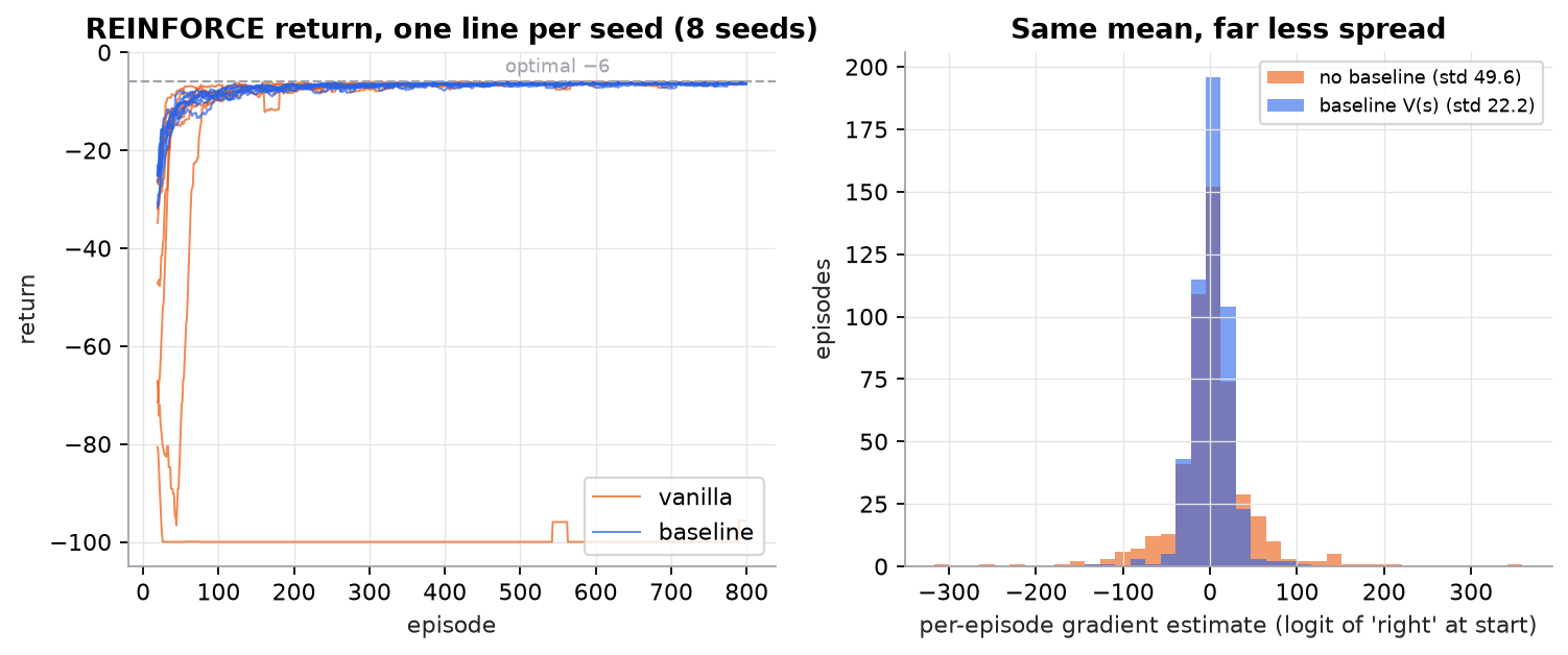
Synthetic 4×4 grid, −1 per move, episodes capped at 100 steps. Left: learning rate 0.02, . Right: both estimators have about the same mean (they are both unbiased), but the baseline halves the spread. Produced by code/26-reinforcement-learning/reinforce.py.
The flat orange line is the classic policy-gradient failure. In that seed a few early updates made "left" at the start cell almost certain, the agent walked into the wall for 100 steps every episode, and since every episode now looked identical, there was nothing left to learn from. The policy collapsed before it found the goal.
Try it (predict first, then edit the script and check):
- Raise
lrfrom 0.02 to 0.05. Predict how many of the 8 vanilla seeds still reach −6, and whether the baseline runs are safer. - Set the baseline to a constant (about the random policy's value at the start) instead of the learned . Predict whether the variance in the right panel shrinks as much as with the per-state values.
- Compute returns from the start of the episode ( for every step) instead of returns-to-go. Predict the effect on the right panel's spread.
- Add an entropy bonus,
+ beta * entropy, withbeta = 0.01. Predict whether the collapsed seed recovers.
3. The math
Symbols
| Symbol | Meaning | Shape / type |
|---|---|---|
| policy parameters (here, one logit per state and action) | ||
| one-hot features of state | ||
| softmax policy, | probability | |
| a trajectory | sequence | |
| expected return of the policy, | scalar | |
| return-to-go from step : | scalar | |
| baseline, any function of the state only | scalar | |
| advantage estimate, | scalar | |
| learning rate | scalar |
The log-derivative trick
We want the gradient of an expectation whose distribution depends on :
We can't sample . But (that is just the chain rule for ), which turns the sum back into an expectation we can sample:
The trajectory probability is a product of policy terms and environment terms, . Its log is a sum, and the environment terms don't depend on , so their gradient is zero. The model of the world drops out:
Rewards before step can't depend on , and dropping them leaves the expectation unchanged, so we keep only returns-to-go. That gives the REINFORCE estimator, averaged over sampled episodes:
Why the baseline is free
For any that doesn't depend on the action:
So subtracting adds zero on average: no bias. The variance does change, and is lowest (roughly) when , which makes an estimate of "how much better than usual was this action". If depended on the action, the third step would fail and the gradient would be biased.
The softmax gradient
For with logits :
With one-hot features, the gradient for is that vector placed in the column of state and zeros elsewhere.
Worked example: one update
A 3-step episode: from cell (2,1) go right to (2,2), right to (2,3), down to the goal. Rewards , , .
Returns-to-go, backward:
- .
- .
- .
Policy at (2,1). Logits for (up, down, left, right) .
- Exponentials: , , , .
- Sum: .
- Probabilities: , , , .
Gradient of with respect to the four logits .
Vanilla step : . The logit of "right" goes down by 0.148, even though right was the best move. Every return here is negative.
With a baseline (the agent usually needs a bit more than 3 moves from there): . Step . Now "right" goes up and the others go down, because this episode beat expectations.
4. Implementation
The full script is code/26-reinforcement-learning/reinforce.py (NumPy only). It uses the same grid and step function as the MDP lesson, with actions numbered 0 to 3.
Build it from scratch
Step 1: the policy. One-hot features times a weight matrix gives four logits; softmax turns them into probabilities. Subtracting the max before exp changes nothing mathematically and prevents overflow.
def softmax(z):
    e = np.exp(z - z.max())  # shift for numerical safety
    return e / e.sum()

def policy(theta, x):
    return softmax(theta @ x)  # theta: [4 actions, 16 features] -> probs: [4]
Predict: with theta all zeros, what does policy return for any state?
Step 2: sample an episode and compute returns-to-go. REINFORCE is on-policy and Monte Carlo: it needs complete episodes from the current policy. The returns-to-go loop is the backward recursion .
def rollout(theta, rng, max_steps=100):
    s, traj = START, []
    for _ in range(max_steps):
        x = features(s)
        p = policy(theta, x)
        a = rng.choice(4, p=p)
        s, r, done = step(s, a)
        traj.append((x, a, r, p))
        if done:
            break
    return traj

def returns_to_go(rewards, gamma):
    G, out = 0.0, []
    for r in reversed(rewards):  # G_t = r_t + gamma * G_{t+1}
        G = r + gamma * G
        out.append(G)
    return out[::-1]
Predict: why does the trajectory store p, the probabilities at sampling time?
Step 3: the gradient. For a softmax over a linear layer, is the outer product of with the features. Each step adds it, weighted by the advantage. The baseline is a linear value function ; it reads only the state, so it can't bias the gradient.
def grad_log_pi(x, a, p):
    """For a softmax over theta @ x: d log pi(a) / d theta = (onehot(a) - p) outer x."""
    g = -p.copy()
    g[a] += 1.0
    return np.outer(g, x)

def episode_gradient(traj, gamma, w=None):
    G = returns_to_go([r for _, _, r, _ in traj], gamma)
    grad = np.zeros((4, N * N))
    for (x, a, _, p), g_t in zip(traj, G):
        adv = g_t - (w @ x if w is not None else 0.0)  # baseline b(s) = w . x does not depend on a
        grad += adv * grad_log_pi(x, a, p)
    return grad, G
Predict: if the policy were already certain ( for the chosen action), what would grad_log_pi be, whatever the return?
Step 4: the training loop. Gradient ascent on expected return, one episode per update. The baseline is fit at the same time by regressing toward the observed returns-to-go: a tiny critic.
def reinforce(episodes, seed, baseline, lr=0.02, lr_v=0.1, gamma=0.99):
    rng = np.random.default_rng(seed)
    theta, w = np.zeros((4, N * N)), np.zeros(N * N)
    curve = []
    for _ in range(episodes):
        traj = rollout(theta, rng)
        grad, G = episode_gradient(traj, gamma, w if baseline else None)
        theta += lr * grad  # gradient ASCENT on expected return
        if baseline:  # fit the baseline: V(s) toward the observed return-to-go
            for (x, _, _, _), g_t in zip(traj, G):
                w += lr_v * (g_t - w @ x) * x
        curve.append(sum(r for _, _, r, _ in traj))
    return theta, curve
Predict: the episode is thrown away after one update. What would go wrong if you kept old episodes and reused them for many updates, as DQN does?
Use the library
In PyTorch you don't write the gradient. You write a loss whose gradient is the policy gradient, and autograd does the rest. The advantages must be constants, so they are detached.
import torch

logits = policy_net(states)                         # [T, n_actions]
logp = torch.log_softmax(logits, dim=-1)
logp_taken = logp.gather(1, actions[:, None]).squeeze(1)   # [T]
adv = (returns - values).detach()                   # baseline from a value net; no gradient through it
adv = (adv - adv.mean()) / (adv.std() + 1e-8)       # per-batch normalization, standard practice
loss = -(logp_taken * adv).mean()                   # minimize the negative = ascend expected return
loss.backward(); optimizer.step(); optimizer.zero_grad()
What the library version adds: autograd through any network, Adam instead of plain SGD, batches of many episodes per update (a far better gradient estimate than one), advantage normalization, and usually an entropy bonus. Libraries such as Stable-Baselines3 don't ship plain REINFORCE; they ship A2C and PPO, which are this loss plus a learned critic and, for PPO, a clipped ratio.
Run it
uv run code/26-reinforcement-learning/reinforce.pyreturns-to-go G_0, G_1, G_2 = [-2.71, -1.9, -1.0]
logits at (2,1) = [ 0. 0.5 -0.5 1. ] softmax probs = [0.1674 0.276 0.1015 0.4551]
grad of log pi(right) w.r.t. the logits = onehot(right) - p = [-0.1674 -0.276 -0.1015 0.5449]
vanilla: step = lr * G_0 * grad = 0.1 * -2.71 * grad = [ 0.0454 0.0748 0.0275 -0.1477]
baseline: A = G_0 - b = -2.71 - (-3.5) = 0.79; step = 0.1 * 0.79 * grad = [-0.0132 -0.0218 -0.008 0.0431]
V(start) under the random policy = -39.41
no baseline: mean = 0.99 std = 49.58
baseline V(s): mean = 1.17 std = 22.24
vanilla mean return, first 100 episodes = -29.57; last 100 per seed = [-99.1 -6.2 -6.2 ...]; seeds within 1 of optimal: 7/8
baseline mean return, first 100 episodes = -13.61; last 100 per seed = [-6.5 -6.2 -6.4 ...]; seeds within 1 of optimal: 8/8The first block is the worked example. The two gradient means differ only by sampling noise (both estimate the same true gradient); the standard deviations differ by more than 2×.
5. Engineering
REINFORCE is the core of LLM RL. Map the pieces:
| RL | LLM fine-tuning |
|---|---|
| state | prompt plus tokens generated so far |
| action | next token |
| policy | the model's next-token distribution |
| trajectory | one sampled response |
| reward | reward-model score or verifier result, usually once at the end |
| sum of the response's token log-probs |
With one reward at the end and , every token's return-to-go is that same reward, so the update is "raise the log-probability of every token in a good response, lower it in a bad one". The baseline matters even more here, since rewards like "tests passed: 1" are all non-negative. GRPO (in fine-tuning in practice) samples a group of responses per prompt and uses the group's mean reward as the baseline (and divides by the group's standard deviation). RLOO uses the mean of the other responses, which keeps the baseline independent of the response being scored. Both are REINFORCE baselines with no learned critic. They then add PPO's clipped ratio and a KL penalty to a reference model for stability.
Variance is the enemy. One episode gives a very noisy gradient. Standard remedies, roughly in order of impact: average over many episodes per update; use returns-to-go; subtract a baseline (a learned value function gives actor-critic); normalize advantages per batch; use a discount below 1 or GAE (in the PPO lesson) to trade a little bias for a lot less variance.
On-policy cost. The gradient formula assumes the data came from the current policy. After one update the data is stale. Reusing it needs importance weights , which can explode; PPO clips them. This is why policy-gradient methods are less sample-efficient than replay-based DQN.
Entropy collapse. As in the figure, a policy can become near-deterministic before it finds good behavior, and then it stops exploring. Monitor policy entropy; add a small entropy bonus; lower the learning rate. In LLM RL the symptom is responses that all look the same within a group, which also makes group-normalized advantages zero.
Watch outFailure modes. Sign errors (descending on the return instead of ascending); letting gradients flow through the baseline or the advantage; a baseline that depends on the action; very large unnormalized returns making steps huge; entropy collapse; reusing old episodes without correction.
Common mistakes
- Using the total episode return for every step instead of returns-to-go, adding noise from rewards the action could not affect.
- Forgetting
.detach()on advantages, so the loss also trains the value network in a strange direction. - Comparing vanilla and baseline runs with one seed each. Policy gradient results vary a lot by seed; plot several.
- Reading a flat learning curve as "converged" when entropy has collapsed and the agent is stuck.
- Thinking the baseline changes what the policy converges to. It changes the noise, not the expected gradient.
6. Knowledge check
Quiz: Policy gradients and REINFORCE
An episode has rewards and . What is the return-to-go ?
Practice exercise. A two-action softmax policy has logits at some state. The agent took action 1 (the second one) and the advantage was . With , what are the new logits, and does the probability of action 1 go up?
Solution
Probabilities: , , sum , so . Gradient of : . Step . New logits . New probability of action 1: . Up from 0.2689.
Implementation challenge. Add a GRPO-style baseline to reinforce.py: for each update, sample 8 episodes with the same policy, compute each episode's total return , and use for every step of episode . Compare learning curves with the learned- baseline over 8 seeds.
Solution sketch
Loop 8 rollouts, collect [sum(r) for each], normalize, then accumulate A_i * grad_log_pi(x, a, p) over all steps of all 8 episodes and divide by 8. No critic is needed. It typically learns in fewer updates than one-episode REINFORCE (each update sees 8× the data) but uses more episodes overall. Its weakness: every step in an episode gets the same advantage, so it can't tell which moves within a long episode were good; a per-state critic can. That is acceptable for LLM responses with one end-of-response reward, which is why GRPO works there.
Summary
- Policy gradients optimize the policy directly: .
- The log-derivative trick turns the gradient of an expectation into an expectation you can sample; the environment's dynamics drop out.
- Returns-to-go and a state-only baseline cut variance without adding bias; a learned value baseline gives actor-critic.
- REINFORCE is on-policy and high-variance: each update needs fresh episodes, and runs can collapse to a deterministic bad policy.
- LLM RL is REINFORCE over tokens: GRPO and RLOO are group baselines, and PPO adds clipping and a KL anchor.
Next: Proximal policy optimization (PPO)
Related: DQN · MDPs · Fine-tuning in practice · Gradient descent
Parts of this lesson are adapted from AI Engineering from Scratch by Rohit Ghumare (MIT license, notice): Policy Gradient — REINFORCE from Scratch.
Interview angle
Derive the policy gradient. Why don't you need a model of the environment?
The objective is J(θ), the expected return over trajectories sampled from the policy. Its gradient is the sum over trajectories of ∇P(τ) times the return. Using ∇P = P ∇log P, that becomes an expectation of ∇log P(τ) times the return, which you can estimate by sampling episodes. The trajectory probability is a product of the start distribution, the policy terms π(a_t | s_t), and the transition terms P(s_{t+1} | s_t, a_t). Taking the log turns it into a sum, and only the policy terms depend on θ, so the transition terms vanish from the gradient. That's why REINFORCE is model-free: you only need to sample from the environment and differentiate log π of the actions you took. Then you replace the full return with returns-to-go, since an action can't affect earlier rewards, and subtract a baseline.
Policy gradients or Q-learning: how do you choose?
Q-learning methods like DQN are off-policy and reuse data through a replay buffer, so they are sample-efficient, but they need a max over actions, which is natural only for a small discrete action set. They also learn a deterministic greedy policy. Policy gradients handle continuous or huge action spaces, since they only need log π of the sampled action, and they represent stochastic policies directly. Their cost is high variance and on-policy data, so they need more samples and careful variance reduction. In practice: discrete actions with expensive data, consider DQN-family; continuous control, PPO or SAC; LLMs, where the action space is the vocabulary and you already have a policy that outputs log-probs, policy gradients through PPO or GRPO. Actor-critic methods sit in the middle by learning both.
Your REINFORCE agent's return goes flat at a bad value early and never improves. What do you check?
First, policy entropy. If it has collapsed, the policy became near-deterministic before finding good behavior: every episode looks the same, the advantages go to zero, and learning stops. The fixes are a lower learning rate, an entropy bonus, and advantage normalization so a few large returns can't slam the logits. Second, the sign and the baseline. Make sure the update ascends the return, that advantages are detached, and that the baseline depends only on the state. Third, scale. Huge unnormalized returns make step sizes explode. Fourth, check several seeds. One stuck seed out of eight is the normal variance of the method, while every seed stuck points to a bug. On a grid, I'd also print the policy at the start state; in my toy run the stuck seed had put probability 1 on walking into a wall.
GRPO samples 4 answers with rewards 1, 0, 0, 1. What are the advantages, and how does that relate to REINFORCE?
The group mean is 0.5. The deviations are +0.5, −0.5, −0.5, +0.5, so the population standard deviation is 0.5, and the normalized advantages are +1, −1, −1, +1. Every token in the two correct answers gets advantage +1, and every token in the wrong ones gets −1. That is REINFORCE with γ = 1, a single terminal reward, and the group mean as the baseline. The baseline is unbiased as long as it doesn't depend on the answer being scored, which is strictly true for leave-one-out versions like RLOO and approximately true for the group mean. If all four answers had the same reward, every advantage would be zero, and the prompt would teach nothing. That's why prompt difficulty and group size matter. GRPO then adds PPO-style ratio clipping and a KL penalty toward a reference model.