Module 26: Reinforcement learning 50 min14 min quick readDeep learning
Proximal policy optimization (PPO)
Compute GAE advantages and PPO's clipped surrogate by hand, implement an actor-critic PPO loop that logs KL and clip fraction, and explain how PPO, its KL penalty, and GRPO are used to fine-tune LLMs.
Before this: Policy gradients and REINFORCE
Quick read: the intuition, interactive visualization, summary, and interview questions. The math, implementation, engineering, and knowledge-check sections are hidden.
Mental model. REINFORCE takes one step per batch of experience and then throws the batch away. PPO wants to squeeze several steps out of each batch, but the more you optimize on old data, the more the policy drifts from the one that collected it, and the less the data means. So PPO puts the policy on a leash: for each action, it stops rewarding changes once the new probability is more than about 20% above or below the old one. Within the leash, optimize freely. Past it, the gradient goes to zero.
You will learn to
- Compute the probability ratio and the clipped surrogate objective by hand, and say when the gradient is zero.
- Compute generalized advantage estimates (GAE) for a short episode, step by step.
- Implement PPO from scratch: rollout, GAE, K epochs of minibatch updates, a critic, approx KL, and clip fraction.
- Read PPO's health metrics and diagnose a run that is updating too hard or too little.
- Explain the RLHF setup (policy, reference, reward, and value models; KL penalty) and how GRPO removes the value model.
Why it matters. PPO (Schulman et al., 2017) became the default deep RL algorithm because it is simple, works across discrete and continuous control, and forgives imperfect hyperparameters. It was the RL step in the original InstructGPT-style RLHF recipe, and GRPO, used for reasoning models, is PPO's clipped objective with a group baseline instead of a critic. If you are asked about RL for LLMs in an interview, PPO's loss is the thing to be able to write on the whiteboard.
1. Intuition
REINFORCE has two weaknesses. Its gradient is noisy, and its data is single-use: after one update the policy has changed, so the episodes no longer come from "the current policy" that the formula assumes.
Reusing data with a ratio. If a batch was collected by an old policy , you can still estimate how a new policy would do by reweighting each sample by . An action the new policy likes twice as much counts twice. This is importance sampling. It is exact on average but becomes very noisy once drifts far from 1, and nothing stops the optimizer from pushing to 10 on one lucky sample.
The clip. PPO caps how much credit you get for moving each probability. For an action with a positive advantage (better than expected), raising its probability helps, but only up to (typically ); past that the objective goes flat and the gradient is zero. For a negative advantage, lowering its probability helps only down to . Moves in the harmful direction are never capped, so the objective always pushes back against mistakes. The result is an approximate trust region with no second-order math (TRPO, PPO's predecessor, needed a constrained optimization with conjugate gradients).
The critic and GAE. PPO is an actor-critic method. The actor is the policy. The critic is a value function , learned by regression, used as the baseline. Instead of the full Monte Carlo return, PPO usually builds advantages with GAE: a weighted blend of one-step, two-step, … lookaheads controlled by . With you trust the critic after one step (low variance, more bias); with you use the real return (no bias from the critic, high variance). is the usual compromise.
The loop. Collect a batch with the current policy, freeze a copy of its log-probabilities, compute advantages, then run epochs of minibatch gradient steps on the clipped objective plus a value loss (and often an entropy bonus). Throw the batch away and repeat.
Key distinctionThe clip does not cap the KL divergence directly. It removes the incentive to move a sampled action's probability further once it is outside . Other actions' probabilities, other states sharing weights, and many epochs can still push the policy far away. That is why you also log the approximate KL and the fraction of clipped samples, and sometimes stop the epoch loop early when KL gets too large.
2. Visualization
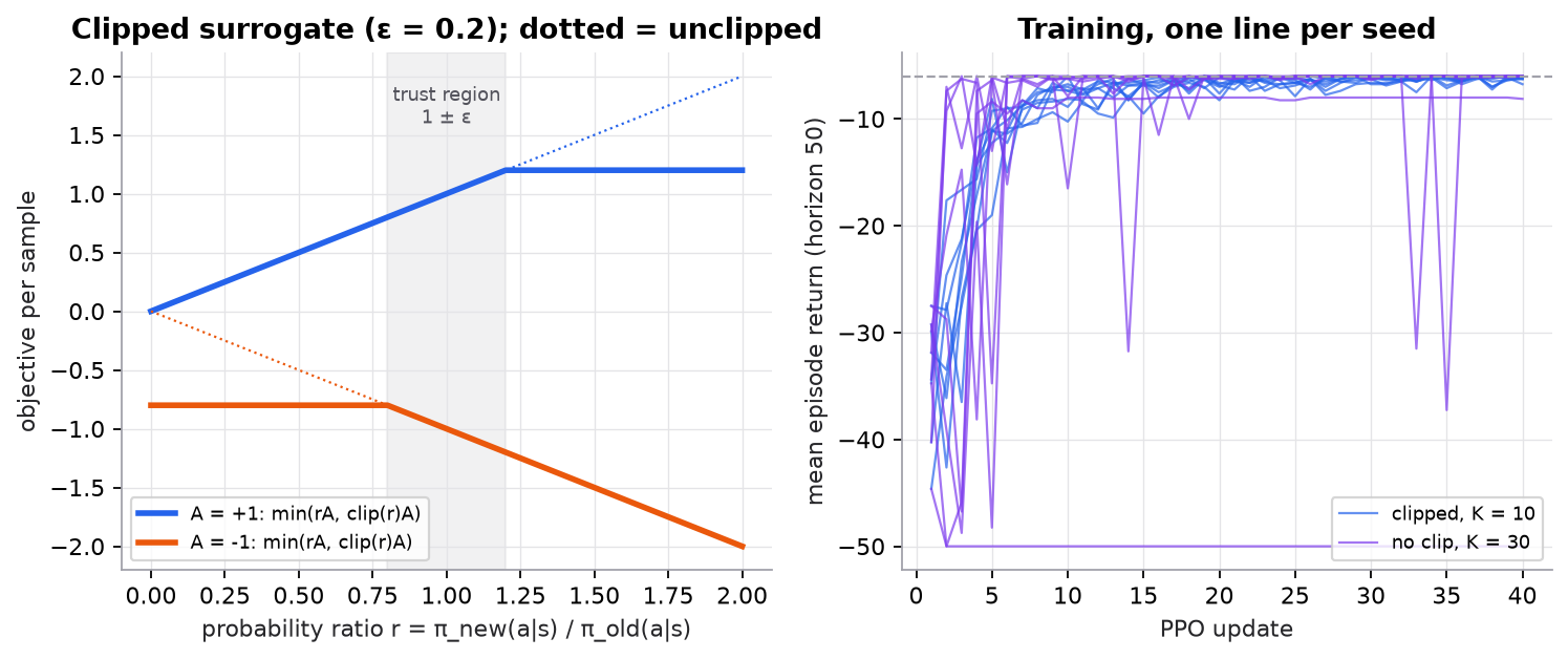
Left: the objective PPO maximizes for one sample. Right: synthetic 4×4 grid, −1 per move, episodes capped at 50 steps; each update uses 8 episodes. Produced by code/26-reinforcement-learning/ppo.py.
Read the left panel as "where is there a gradient?". On the blue line the slope is positive until and zero after. On the orange line the slope is zero until and negative after. The flat parts are where the clip stops the optimizer.
The right panel shows why that matters. Without the clip and with 30 epochs per batch, the approximate KL between consecutive policies averages 1.7 to 3.3 over the first five updates, against at most 0.09 (seed average) for clipped PPO. On this tiny grid most unclipped runs get lucky and learn fast, but one seed jumps to a policy that never reaches the goal in 50 steps (return −50) and never recovers, since every later episode is identical and carries no learning signal.
Try it (predict first, then edit the script and check):
- Set . Predict the clip fraction and the speed of learning compared with .
- Keep but set
epochs=30. Predict whether the clip alone keeps every seed stable, and what happens to the clip fraction. - Set GAE's
lam=1.0and thenlam=0.0. Predict which learns faster early on, when the critic is still wrong. - Remove the advantage normalization line in
ppo_update. Predict what happens to the effective step size as returns shrink from −50 to −6.
3. The math
Symbols
| Symbol | Meaning | Shape / type |
|---|---|---|
| current policy; frozen policy that collected the batch | distributions over 4 actions | |
| probability ratio | scalar per sample | |
| advantage estimate for sample | scalar per sample | |
| clip range | scalar, usually 0.2 | |
| critic (value function) with parameters | scalar per state | |
| TD error | scalar | |
| discount; GAE mixing parameter | scalars in | |
| weights on the value loss and entropy bonus | scalars, often 0.5 and 0.0 to 0.01 | |
| epochs per batch; minibatch size | integers |
The clipped surrogate
The ratio is computed in log space, , for numerical stability. At (before any update) the gradient of equals , exactly the REINFORCE gradient. PPO's full loss to minimize is
where is the value target and is entropy.
Generalized advantage estimation
At a true terminal state, . If the episode was only cut off by a time limit, use the critic's estimate of the last state instead.
Worked example 1: the clip
, so the clip range is .
| min | gradient? | ||||
|---|---|---|---|---|---|
| 1.1 | +2 | 2.20 | yes, inside the range | ||
| 1.5 | +2 | 2.40 | no: already raised enough | ||
| 0.7 | +2 | 1.40 | yes: a good action was made less likely, push back | ||
| 0.7 | −1 | −0.80 | no: already lowered enough | ||
| 1.5 | −1 | −1.50 | yes: a bad action was made more likely, push back |
When the min picks the clipped term, that term is a constant in and the gradient is zero. The min is pessimistic: it always takes the lower of the two estimates.
Worked example 2: GAE on three steps
An episode from a cell near the goal takes three moves, rewards , and ends at the goal. The critic currently says for the three states visited. , , so .
TD errors:
- (the next state is terminal, value 0).
- .
- .
Advantages, backward:
- .
- .
- .
Value targets : , , . The critic was too optimistic in every state (actual returns were worse), so every advantage is negative and the critic will be pulled down.
4. Implementation
The full script is code/26-reinforcement-learning/ppo.py (NumPy only). The policy is the same softmax over a logit table as in REINFORCE; the critic is a linear value on one-hot states. With a table, each weight only affects one state, which is why a learning rate as large as 4.0 is stable here; a neural network would use something like with Adam.
Build it from scratch
Step 1: collect a rollout. Run the current policy for 8 episodes. If an episode hits the 50-step horizon without reaching the goal, it was truncated, not terminated, so we record the critic's value of the last state for bootstrapping.
def collect(theta, w, rng, n_episodes=8, horizon=50):
    eps = []
    for _ in range(n_episodes):
        s, X, A, R = START, [], [], []
        done = False
        for _ in range(horizon):
            x = features(s)
            a = rng.choice(4, p=probs(theta, x[None])[0])
            s, r, done = step(s, a)
            X.append(x), A.append(a), R.append(r)
            if done:
                break
        last_v = 0.0 if done else w @ features(s)  # truncated by the horizon: bootstrap, don't pretend it ended
        eps.append((np.array(X), np.array(A), np.array(R), last_v))
    return eps
Predict: if you set last_v = 0.0 for truncated episodes too, would the critic's values come out too high or too low?
Step 2: GAE. One backward pass computes every TD error and accumulates them with weight , exactly as in worked example 2. The value targets are advantages plus the values used to compute them.
def gae(rewards, values, last_v, gamma=0.99, lam=0.95):
    """delta_t = r_t + gamma V(s_{t+1}) - V(s_t);  A_t = delta_t + gamma*lam*A_{t+1}."""
    adv, running = np.zeros(len(rewards)), 0.0
    next_v = last_v
    for t in reversed(range(len(rewards))):
        delta = rewards[t] + gamma * next_v - values[t]
        running = delta + gamma * lam * running
        adv[t], next_v = running, values[t]
    return adv, adv + values  # advantages, value targets (returns)
Predict: with lam=1.0 and a critic that is all zeros, what do the advantages equal?
Step 3: the ratio and the clip mask. For each minibatch, compute new log-probs, the ratio against the frozen old ones, and which samples still have a gradient. A sample is "clipped" when it is already past the edge in the direction its advantage wants.
p = probs(theta, X[j])
logp = np.log(p[np.arange(len(j)), A[j]])
ratio = np.exp(logp - logp_old[j])  # new / old, computed in log space
# The gradient flows only where the min picks the unclipped term.
active = ~(((adv[j] > 0) & (ratio > 1 + eps)) | ((adv[j] < 0) & (ratio < 1 - eps)))
clipped += (~active).sum()
seen += len(j)
Predict: on the very first minibatch of the first epoch, what fraction of samples is clipped, and why?
Step 4: the gradient step. The gradient of with respect to the logits is . Multiply by the mask, average over the minibatch, and ascend. The critic takes a regression step toward the value targets in the same loop.
g = -p
g[np.arange(len(j)), A[j]] += 1.0  # d log pi(a) / d logits
coef = (active * ratio * adv[j])[:, None]  # d(ratio * A) / d logits = ratio * A * (onehot - p)
theta += lr * (coef * g).T @ X[j] / len(j)  # ascend the surrogate
w += lr_v * ((ret[j] - X[j] @ w)[:, None] * X[j]).mean(axis=0)  # critic: regress to targets
Predict: if you dropped the ratio * factor, which earlier algorithm would each step become?
Step 5: the outer loop and the health metrics. Normalize advantages per batch, run epochs over shuffled minibatches, then measure how far the policy moved. mean(logp_old - logp_new) over the batch's own samples estimates .
adv = (adv - adv.mean()) / (adv.std() + 1e-8)  # per-batch advantage normalization
n, clipped, seen = len(A), 0, 0
for _ in range(epochs):
    order = rng.permutation(n)
    for i in range(0, n, batch):
        j = order[i:i + batch]
        ...  # steps 3 and 4
p = probs(theta, X)
logp_new = np.log(p[np.arange(n), A])
approx_kl = np.mean(logp_old - logp_new)  # estimate of KL(old || new) on the rollout's samples
Predict: if approx KL comes out negative on some update, is that a bug?
Use the library
For control tasks, Stable-Baselines3 implements PPO with these defaults spelled out (it needs PyTorch, so this snippet is not run here):
import gymnasium as gym
from stable_baselines3 import PPO

env = gym.make("CartPole-v1")
model = PPO("MlpPolicy", env, n_steps=2048, batch_size=64, n_epochs=10,
            gamma=0.99, gae_lambda=0.95, clip_range=0.2, ent_coef=0.0, vf_coef=0.5,
            target_kl=None, seed=0, verbose=1)
model.learn(total_timesteps=100_000)   # logs approx_kl, clip_fraction, entropy_loss, explained_variance
What it adds over our script: neural actor and critic (shared or separate), Adam, gradient-norm clipping (max_grad_norm), vectorized environments, optional value-function clipping, optional early stopping when KL exceeds target_kl, and the same metrics we log. For LLMs, Hugging Face's TRL library provides PPO and GRPO trainers that handle generation, the reference model, reward scoring, and per-token KL; check the current docs for their exact configuration classes, which change between versions.
Run it
uv run code/26-reinforcement-learning/ppo.pyr = 1.5, A = +2.0: min(+3.00, +2.40) = +2.40 (clipped, gradient 0)
r = 0.7, A = -1.0: min(-0.70, -0.80) = -0.80 (clipped, gradient 0)
advantages = [-0.456 -0.185 -0.1 ] value targets = [-2.956 -1.985 -1. ]
=== PPO: 40 updates x (8 episodes, horizon 50), K = 10 epochs, minibatch 64, lr 4.0, 8 seeds ===
update 1: mean return = -34.06 approx KL = 0.0662 clip fraction = 0.28
update 10: mean return = -7.72 approx KL = 0.0858 clip fraction = 0.17
update 40: mean return = -6.23 approx KL = 0.0031 clip fraction = 0.05
seed 0 critic V(start) = -6.13 (true value of the optimal policy with gamma 0.99: -5.85)
=== Too aggressive: same run with K = 30 epochs and no clipping (epsilon = 100) ===
update 1: mean approx KL = 1.691 (PPO with clipping: 0.066)
clipped, K=10: final mean return per seed (last 5 updates) = [-6.3 -6.4 -6.2 -6.3 -6.4 -6.3 -6.2 -6.3]
no clip, K=30: final mean return per seed (last 5 updates) = [ -6. -6. -6.1 -50. -8. -6. -6. -6. ]The first lines match the two worked examples. Clipped PPO's seed-averaged KL stays below 0.1 per update, and its clip fraction falls as the policy settles. Clipped runs end slightly below −6 because the policy stays a little stochastic.
5. Engineering
Healthy PPO numbers. Watch four things per update: mean return, approx KL (often 0.01 to 0.05 per update for neural policies; much higher means steps are too big), clip fraction (roughly 0.1 to 0.3; near 0 means updates are timid or the learning rate is tiny, near 0.5 means the policy is being pushed hard against the clip), and policy entropy (should fall slowly, not crash). For the critic, explained variance near 1 means it predicts returns well.
Hyperparameters that matter. ; = 3 to 10 epochs (more epochs drift further, and the clip doesn't fully stop it); advantage normalization on; a linearly decaying learning rate; GAE ; enough parallel environments that each batch covers varied states. Reward scale matters because the advantage scale sets the step size; normalize rewards or advantages.
PPO for LLMs (RLHF). The classic RLHF recipe (as in InstructGPT) runs PPO with four models:
| Model | Role | Trained? |
|---|---|---|
| Policy | the LLM being tuned; actions are tokens | yes |
| Reference | a frozen copy of the starting (SFT) model | no |
| Reward model | scores a full response, trained on human preference pairs | no (trained earlier) |
| Value model | the critic, predicts reward-to-go per token | yes |
The reward for a response is the reward model's score at the last token, minus a per-token KL penalty at every token. The KL term stops the policy from drifting into text the reward model scores highly but that is gibberish or sycophantic, which is reward hacking. GAE then runs over tokens with . Holding four large models in memory and tuning this loop is expensive, which is why many teams moved to DPO for preference data (see adapting LLMs).
GRPO drops the critic. For each prompt, GRPO samples a group of responses, scores them, and uses each response's group-normalized reward as the advantage for every token in it. That is a REINFORCE group baseline in place of a learned value model. It keeps PPO's clipped ratio and adds a KL term to the reference model directly in the loss. One fewer large model to train, and it works well when rewards come from a verifier (unit tests, exact math answers). The worked GRPO numbers are in fine-tuning in practice.
Watch outFailure modes. Flipped sign (minimizing the surrogate); computing the ratio as
new / oldin probability space (underflow) instead of from log-probs; forgetting to freezelogp_oldbefore the epochs start, so the ratio is always 1 and the clip never acts; bootstrapping past real terminal states, or not bootstrapping on truncation; too many epochs; reward-model hacking in RLHF when the KL coefficient is too small.
Common mistakes
- Believing the clip guarantees a small KL. It only removes the incentive for sampled actions past the edge; log KL and stop early if it spikes.
- Recomputing
logp_oldafter each epoch. It must come from the policy that collected the data. - Leaving advantages unnormalized, so the effective step size changes as returns change.
- Sharing one network for actor and critic without weighting the value loss, so the value gradient swamps the policy gradient.
- In RLHF, judging success by reward-model score alone. Rising reward with rising KL and falling human ratings means the policy is exploiting the reward model.
6. Knowledge check
Quiz: Proximal policy optimization (PPO)
With , a sample has ratio and advantage . What is ?
Practice exercise. With , compute the clipped objective for and , and say whether each has a gradient.
Solution
: unclipped ; clipped ; min , the clipped term, so no gradient. : is inside , so both terms are ; min , and the gradient flows (lowering this bad action's probability further still helps, until ).
Implementation challenge. Add early stopping to ppo_update: after each epoch, compute approx KL on the whole batch, and stop the epoch loop if it exceeds target_kl = 0.02. Then rerun the "no clip, K = 30" configuration with early stopping on. Does it still produce a collapsed seed?
Solution sketch
Move the KL computation inside the epoch loop (after the minibatch loop) and break when it exceeds the target. With no clip, early stopping becomes the only leash: most updates stop after one or two epochs, the per-update KL drops by an order of magnitude, and the collapsing seed typically behaves like the others. This is a KL-constrained update in the spirit of TRPO, done with a cheap check instead of a constrained optimizer. Libraries expose it as target_kl.
Summary
- PPO reuses each batch for several epochs, using the ratio to correct for the policy having changed.
- The clipped surrogate removes the gradient once a sampled action has moved more than in the direction its advantage wants; harmful moves are never clipped.
- GAE blends multi-step TD errors with to trade variance for bias; a learned critic provides the baseline.
- Log approx KL, clip fraction, entropy, and explained variance; too many epochs or too large a learning rate show up there first.
- In RLHF, PPO tunes the LLM against a reward model with a per-token KL penalty to a frozen reference; GRPO drops the value model and uses group-normalized rewards as advantages.
Next: Tokenization and pretraining
Related: Policy gradients and REINFORCE · DQN · Adapting LLMs
Go deeper, code-first (AI Engineering from Scratch): Actor-Critic — A2C and A3C · RL for Games — AlphaZero, MuZero, and the LLM-Reasoning Era
Parts of this lesson are adapted from AI Engineering from Scratch by Rohit Ghumare (MIT license, notice): Proximal Policy Optimization (PPO).
Interview angle
Write down PPO's objective and explain what the clip does, case by case.
The objective is the expectation of min(r·A, clip(r, 1 − ε, 1 + ε)·A), where r is the ratio of the new policy's probability for the sampled action to the old policy's, and A is the advantage. When A is positive, raising the action's probability helps, but once r passes 1 + ε the clipped term is smaller and the min picks it. That term is constant in θ, so the gradient is zero. When A is negative, lowering the probability helps only down to 1 − ε. In the other direction, a good action made less likely or a bad action made more likely, the unclipped term is smaller and the gradient pushes back fully. So the clip limits how far one batch can move the policy in the beneficial direction, a cheap approximate trust region. Add a value loss, maybe an entropy bonus, and run K epochs of minibatches per batch.
PPO, GRPO, or DPO for aligning an LLM: how do you choose?
DPO when I have fixed preference pairs and want something simple. It's an offline classification-style loss with only the policy and a frozen reference, so there's no sampling loop and no reward model to keep around. PPO-based RLHF when I need online learning against a learned reward model and can afford four models: policy, reference, reward, and value. It can improve beyond the static dataset, but it's the most expensive and fiddly option. GRPO when rewards can be checked by a program, like unit tests or exact math answers. It samples several responses per prompt and uses the group-normalized reward as the advantage, so there's no critic, and it keeps PPO's clip plus a KL term to the reference. For reasoning tasks with verifiers, GRPO-style RL is the common choice today. For tone and helpfulness from preference data, DPO is usually the first thing I try.
Your PPO run's approx KL jumps to 0.5 per update and returns become erratic. What do you check?
The policy is moving far more than PPO intends per update, so the ratio-corrected estimates stop meaning anything. In order: the learning rate, which is the most common cause, so I lower it or add linear decay. The number of epochs, since many epochs over one batch drift far even with the clip. Then whether logp_old is actually frozen before the epochs start and computed in log space. Then whether advantages are normalized, because a large reward scale means large steps. Then the clip range itself. I'd also set target_kl to stop an update's epochs early when KL passes something like 0.02, and check gradient-norm clipping. In RLHF the equivalent symptom is the KL to the reference running away while reward-model score climbs. That's usually reward hacking, so I'd raise the KL coefficient and inspect samples.
Compute the GAE advantage for the last two steps of an episode: rewards −1, −1; values 1.8 and 0.9 below zero; terminal after; γ = 0.99, λ = 0.95.
Work backward. The last state is terminal, so its next value is 0. The last TD error is −1 + 0 − (−0.9) = −0.1, and that's also the last advantage. The step before has TD error −1 + 0.99 × (−0.9) − (−1.8) = −1 − 0.891 + 1.8 = −0.091. Its advantage is −0.091 + γλ × (−0.1), with γλ = 0.9405, so −0.091 − 0.09405 = −0.18505. The value targets are the advantages plus the values: −1.98505 and −1.0. Both advantages are negative because the critic was too optimistic, so the actor makes those actions slightly less likely and the critic moves its estimates down. With λ = 0, each advantage would just be its own TD error, −0.091 and −0.1. With λ = 1 it would be the full Monte Carlo return minus the value.