Module 26: Reinforcement learning 40 min11 min quick readDeep learning
MDPs, states, actions, and rewards
Frame a sequential decision problem as a Markov decision process, compute discounted returns and state values with the Bellman equation, and spot broken formulations before training.
Before this: Learning paradigms, Probability and statistics
Quick read: the intuition, interactive visualization, summary, and interview questions. The math, implementation, engineering, and knowledge-check sections are hidden.
Mental model. Reinforcement learning is a game against a world you can't see the rules of. At each turn you look at the board (the state), make a move (the action), and the world hands you a score (the reward) and a new board. A Markov decision process writes those rules down. Every RL algorithm, from tabular Q-learning to the PPO loop that tunes a chat model, is a different way of finding good moves in that same game.
You will learn to
- Name the five parts of an MDP (states, actions, transitions, rewards, discount) for a real problem.
- Compute a discounted return and explain the effective horizon .
- Define a policy, a state value , and an action value , and check a value with the Bellman equation by hand.
- Run policy evaluation and value iteration on a small grid.
- Diagnose common formulation bugs: a non-Markov state, sparse or hackable rewards, an unbounded return.
Why it matters. Supervised learning gives you the right answer for every input. Reinforcement learning gives you only a score, often late, for a whole sequence of choices. Before any algorithm can learn from that, the problem needs a precise shape. Most "RL doesn't work" bugs are formulation bugs: the state is missing information, the reward rewards the wrong thing, or the return is infinite. The same shape underlies RLHF and GRPO-style fine-tuning, where the state is the text so far and each action is the next token.
1. Intuition
Picture a robot on a 4×4 floor. It starts in the top-left corner and wants to reach the charger in the bottom-right corner. Each move drains a little battery, so every step costs . Bumping into a wall wastes the move. The episode ends at the charger.
That is a complete RL problem. Five things define it:
| Piece | In the grid | In an LLM fine-tuning loop |
|---|---|---|
| State | which cell the robot is in | the prompt plus the tokens generated so far |
| Action | up, down, left, right | the next token |
| Transition | the cell you land in | append the token (deterministic) |
| Reward | per move | usually 0 until the end, then a reward-model score or a verifier's pass/fail |
| Discount | how much later rewards count | often 1, since responses are finite |
The agent's behavior is a policy : for each state, a probability for each action. The goal is a policy that collects as much total reward as possible, not just the best next reward. That difference is the heart of RL: a move can look bad now (a detour) and be right overall.
The Markov property. The next state depends only on the current state and action, not on how you got there. In the grid that holds: the cell is all you need. When it fails, the fix is in the state, not the algorithm. A single frame of a video game hides which way the ball is moving, so DQN stacked the last four frames into one state. A chat model's state is the full context window for the same reason.
Discounting. A reward steps in the future is multiplied by . With a reward 10 steps away keeps about a third of its weight; 50 steps away it is nearly gone. A rough rule: buys a horizon of about steps.
Key distinctionReward vs return vs value. A reward is the single number from one step. The return is the discounted sum of rewards from now to the end of one episode. A value is the expected return, averaged over everything the policy and world might do. Algorithms learn values; you observe rewards.
2. Visualization
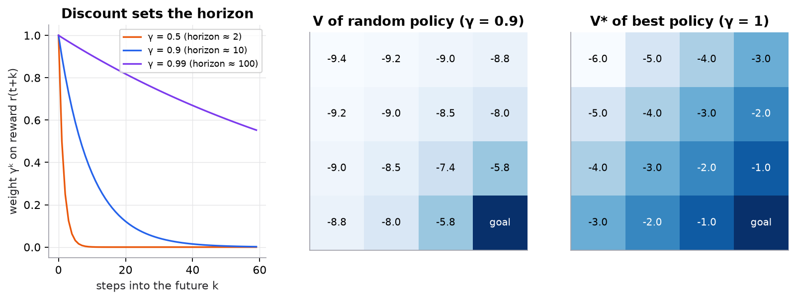
Synthetic 4×4 grid, every move costs −1. Left: how fast each discount forgets the future. Middle: a random walker expects to pay a lot before stumbling onto the goal. Right: the best policy pays exactly the number of moves it needs.
Try it (predict first, then run code/26-reinforcement-learning/mdp.py):
- In the middle panel, why are the two cells next to the goal equal (−5.8), and why is the start corner worst? Predict what happens to the start corner if you change to 0.99.
- The random policy's mean undiscounted return over 5,000 rollouts is about −60 even though the optimum is −6. Predict whether the standard deviation is small or large, then check the script output.
- In the right panel, values go up by exactly 1 per step toward the goal. What would change if one interior cell were a wall?
- Change the step reward to −2. Predict the new at the start, and whether the best policy changes.
3. The math
Symbols
| Symbol | Meaning | Shape / type |
|---|---|---|
| set of states, set of actions | finite sets here (16 cells, 4 moves) | |
| state, action, reward at step | one cell, one move, scalar | |
| transition probability | table | |
| discount factor | scalar in | |
| policy: probability of action in state | , rows sum to 1 | |
| return from step | scalar | |
| state value: expected return from under | vector, length | |
| action value: expected return taking in , then following | ||
| optimal values (best policy) | same shapes |
Return and values
If every reward is bounded by and , then , which is where the "horizon" comes from.
The Bellman equations
Split the return into "this step" plus "everything after", then take expectations:
The first (expectation) equation averages over the policy's actions; it defines the value of a fixed policy. The second (optimality) equation takes the best action; its solution is the value of the best policy. Policy evaluation repeats the first as an update until nothing changes. Value iteration repeats the second. Both converge for (and here for too, because every policy that matters reaches the terminal state).
Worked example 1: a discounted return
Six moves to the goal, each reward , :
- Powers: , , , .
- Sum: .
- . Check with the geometric-series formula: . ✓
With the same path returns ; with it returns , so a short horizon barely tells a 6-step path from a 60-step one.
Worked example 2: checking a value with the Bellman equation
Uniform random policy ( for each action), . Take the cell , just left of the goal. The script's converged values for the cells each action reaches:
| action | next cell | ||
|---|---|---|---|
| up | (2, 2) | −7.416 | |
| down | (3, 2), wall bump | −5.757 | |
| left | (3, 1) | −7.970 | |
| right | (3, 3), goal | 0 |
- Sum of the last column: .
- Multiply by : .
- That equals from the table. ✓ The value is a fixed point: plug it in on the right and it comes back out on the left.
For the optimal values with : , and by the same rule each step away from the goal subtracts 1, giving .
4. Implementation
The full script is code/26-reinforcement-learning/mdp.py (NumPy only). It builds the grid, rolls out a random policy, and solves for values two ways.
Build it from scratch
Step 1: the world. The environment is one function: given a state and action, return the next state, the reward, and whether the episode ended. Writing transitions and rewards in code, not a table, is how most simulators work. Clamping the coordinates is the "bump into the wall" rule.
N = 4
STATES = [(r, c) for r in range(N) for c in range(N)]
ACTIONS = {"up": (-1, 0), "down": (1, 0), "left": (0, -1), "right": (0, 1)}
START, GOAL = (0, 0), (3, 3)

def step(s, a):
    if s == GOAL:
        return s, 0.0, True                     # absorbing terminal state
    dr, dc = ACTIONS[a]
    s2 = (min(max(s[0] + dr, 0), N - 1), min(max(s[1] + dc, 0), N - 1))
    return s2, -1.0, s2 == GOAL
Predict: what does step((0, 0), "up") return?
Step 2: the return. Working backward turns the infinite sum into one multiply-add per step, using . Every RL codebase has this loop somewhere (it reappears as "returns-to-go" in policy gradients).
def discounted_return(rewards, gamma):
    g = 0.0
    for r in reversed(rewards):   # G_t = r_t + gamma * G_{t+1}
        g = r + gamma * g
    return g
Predict: discounted_return([0, 0, 0, 1], 0.5)?
Step 3: a policy and a rollout. A policy maps a state to a distribution over actions. A rollout samples from it until the episode ends. Averaging many rollouts estimates the value by brute force (this is the Monte Carlo method).
def uniform(_s):
    return {a: 0.25 for a in ACTIONS}

def rollout(policy, rng, max_steps=500):
    s, rewards = START, []
    for _ in range(max_steps):
        dist = policy(s)
        a = rng.choices(list(dist), weights=list(dist.values()))[0]
        s, r, done = step(s, a)
        rewards.append(r)
        if done:
            break
    return rewards
Predict: why does rollout need max_steps even though this grid always reaches the goal eventually?
Step 4: policy evaluation. Apply the Bellman expectation equation to every state, over and over, until the largest change is tiny. Updating V in place (using new values as soon as they exist) converges a bit faster than keeping two copies.
def policy_evaluation(policy, gamma, tol=1e-10):
    V = {s: 0.0 for s in STATES}
    while True:
        delta = 0.0
        for s in STATES:
            if s == GOAL:
                continue
            v = sum(p * (r + gamma * V[s2]) for a, p in policy(s).items() for s2, r, _ in [step(s, a)])
            delta, V[s] = max(delta, abs(v - V[s])), v
        if delta < tol:
            return V
Predict: with gamma=1.0 and the uniform policy, this still converges. Would it converge on a grid with no reachable goal?
Step 5: value iteration. Replace the average over the policy with a max over actions. The result is , and acting greedily on it is optimal.
def value_iteration(gamma, tol=1e-10):
    V = {s: 0.0 for s in STATES}
    while True:
        delta = 0.0
        for s in STATES:
            if s == GOAL:
                continue
            v = max(r + gamma * V[s2] for a in ACTIONS for s2, r, _ in [step(s, a)])
            delta, V[s] = max(delta, abs(v - V[s])), v
        if delta < tol:
            return V
Predict: how many sweeps until reaches −6, if each sweep goes in row-major order from (0,0)?
Use the library
Gymnasium is the standard environment interface. Its FrozenLake-v1 is a 4×4 grid MDP like ours, but slippery by default (stochastic transitions), and it exposes the transition table as env.unwrapped.P[s][a], a list of (prob, next_state, reward, done) tuples.
import gymnasium as gym

env = gym.make("FrozenLake-v1", is_slippery=True)
obs, info = env.reset(seed=0)
obs, reward, terminated, truncated, info = env.step(env.action_space.sample())
P = env.unwrapped.P          # P[s][a] -> [(prob, s2, r, done), ...]; plug into the Bellman update
The library adds what our script left implicit: separate terminated (the MDP ended) and truncated (a time limit cut it off) flags, seeded resets, and a standard step signature every RL library understands. The difference between the two flags matters: on truncation you should still bootstrap from the next state's value; on termination you should not.
Run it
uv run code/26-reinforcement-learning/mdp.pygamma = 0.9: G = -4.6856
mean return = -59.87, std = 51.37 (optimal = -6)
Bellman check at (3, 2), gamma=0.9: ... 0.25 * sum(-1 + 0.9 V) = -5.757 = V(3, 2) = -5.757
=== V* by value iteration (gamma = 1): minus the number of moves to the goal ===
[[-6. -5. -4. -3.]
...
saved figures/mdps-states-actions-rewards.png5. Engineering
Write the MDP down before writing code. For each problem, fill in five lines: state, action, transition (known or only sampled?), reward (when, and of what), and or horizon.
| Problem | State | Action | Reward | Discount |
|---|---|---|---|---|
| Robot locomotion | joint angles and velocities | continuous torques | forward progress minus energy | 0.99 |
| Board game | board (plus history if rules need it) | a legal move | +1 win, −1 loss, at the end | 1 (finite game) |
| Inventory | stock level, recent demand | order quantity | revenue minus holding and stockout cost | 0.95 to 0.99 |
| LLM RLHF | prompt plus tokens so far | next token | reward-model score at the end, minus a KL penalty | 1 |
| LLM RL with verifiable rewards | prompt plus tokens so far | next token | 1 if the answer checks out, else 0 | 1 |
Known model vs samples only. If you can write and as tables (small planning problems, games with known rules), dynamic programming like value iteration solves the MDP exactly. Most real problems only let you sample transitions, which is why the next lessons learn from experience.
Reward design is product design. The agent optimizes exactly the number you give it. A boat-racing agent from OpenAI (2016) learned to circle a lagoon collecting point pickups forever instead of finishing the race, because the score rewarded pickups. LLMs trained against a reward model learn to please the reward model (longer answers, confident tone) unless something checks them. Define reward from the outcome you want, and keep a held-out check the agent can't see.
Sparse rewards. If reward only comes at the very end (win or lose), a random policy may never see a nonzero signal. Options: shape the reward with intermediate signals (carefully, since shaping can be hacked), start from a supervised or imitation-learned policy (this is why LLM RL starts from an SFT model), or use a curriculum of easier tasks.
Watch outFailure modes. A state that hides needed information (the agent can't tell two situations apart and dithers); a reward that measures a proxy; on a task that never ends (values become infinite); rewards on wildly different scales (+1000 for one event, ±1 for others), which make value and gradient estimates noisy.
Common mistakes
- Confusing reward with return or value, and comparing a single episode's return to a value estimate as if they should match.
- Using with no time limit or terminal state.
- Treating a time-limit cutoff as a real terminal state, which teaches the agent that the world ends at step 200.
- Leaving information out of the state (velocity, the last few observations, remaining budget) and blaming the algorithm.
- Changing the reward and comparing returns across runs as if the numbers meant the same thing.
6. Knowledge check
Quiz: MDPs, states, actions, and rewards
An episode gives rewards with . What is the return ?
Practice exercise. An episode gives rewards and . Compute , then .
Solution
Work backward. . . . . Directly: . ✓
Implementation challenge. Make the grid slippery: an action moves in the intended direction with probability 0.8 and in each of the two perpendicular directions with probability 0.1. Change step to return a list of (prob, next_state, reward, done) and update value_iteration to sum over it. Does get better or worse than −6, and does the best path change?
Solution sketch
In the Bellman update replace r + gamma * V[s2] with sum(p * (r + gamma * V[s2]) for p, s2, r, _ in outcomes(s, a)). drops below −6 (about −7.4 with ), because slips waste moves. On this open grid the best actions stay "down or right", since a sideways slip along a wall just bumps in place; with pits nearby the best path would move away from them.
Summary
- An MDP is states, actions, transitions, rewards, and a discount. The Markov property says the state carries everything needed to predict what happens next.
- The return is the discounted sum of future rewards; sets an effective horizon of about steps.
- Values are expected returns: for a state, for a state and first action.
- The Bellman equation splits a value into one step of reward plus the discounted value of where you land. Iterating it gives policy evaluation (average) or value iteration (max).
- Most RL failures start in the formulation: missing state, a hackable or sparse reward, or an unbounded return.
Next: Q-learning and SARSA
Related: Learning paradigms · Policy gradients and REINFORCE · Fine-tuning in practice
Go deeper, code-first (AI Engineering from Scratch): Dynamic Programming — Policy Iteration & Value Iteration
Parts of this lesson are adapted from AI Engineering from Scratch by Rohit Ghumare (MIT license, notice): MDPs, States, Actions & Rewards.
Interview angle
Formalize a problem as an MDP. What are the pieces, and what does the Markov property buy you?
An MDP is a tuple of states, actions, a transition distribution P(s′ | s, a), a reward function, and a discount γ. The agent picks actions with a policy π(a | s), and the goal is the policy that maximizes expected discounted return. The Markov property says the next state and reward depend only on the current state and action, not the history. That is what makes the Bellman recursion valid: the value of a state can be written as one step of reward plus the discounted value of the next state, with no need to remember the path. If the property fails, say a single game frame hides velocity, I fix the state, for example by stacking recent frames or using a recurrent network, rather than changing the algorithm. For an LLM the state is the whole context, which is Markov by construction.
How do you choose the discount factor, and what goes wrong at the extremes?
γ trades off near and far rewards, and its practical meaning is a horizon of about 1/(1 − γ) steps: 0.9 looks about 10 steps ahead, 0.99 about 100. Too small and the agent is myopic: it can't tell a 6-step path from a 60-step one, since both look nearly the same after heavy discounting. Too large and credit assignment gets noisy, because many early actions share responsibility for a distant reward, so value estimates have high variance and learn slowly. γ = 1 is only safe when episodes are guaranteed to end, otherwise returns can be infinite. In practice control tasks use 0.99, short finite tasks like LLM responses often use 1, and I tune γ alongside the episode length rather than treating it as fixed.
Your RL agent finds a way to score high reward while doing something useless. How do you diagnose and fix it?
That is reward hacking: the agent optimizes the reward I wrote, not the outcome I wanted. I first watch episodes, not just the curve, and log reward components separately to see which one it is exploiting. Then I check the reward against the true goal on held-out evaluations that the agent never trains on, ideally human review or a different metric. Fixes, in order: redefine the reward from the outcome rather than a proxy, remove or cap the exploited shaping term, add constraints or penalties for the bad behavior, and for LLMs keep a KL penalty to the reference model so the policy can't drift far to exploit reward-model blind spots. I also retrain or ensemble the reward model on the new failure cases, since a fixed learned reward will be exploited again.
Every move costs −1 and the goal is 6 moves away. What are the optimal value at the start with γ = 1 and with γ = 0.9?
With γ = 1 the return is just the sum of six −1 rewards, so V* at the start is −6. With γ = 0.9 the return is −(1 + 0.9 + 0.81 + 0.729 + 0.6561 + 0.59049), which sums to −4.6856; the closed form is −(1 − 0.9⁶)/(1 − 0.9) = −(1 − 0.531441)/0.1. The best policy doesn't change with γ here, since a shorter path is better under any discount when every step costs the same. A follow-up I'd mention: if instead the only reward were +1 at the goal and 0 elsewhere, γ = 1 would make every path that eventually reaches the goal equally good, so you need γ < 1 or a step cost to prefer the short path.