Module 26: Reinforcement learning 45 min12 min quick readDeep learning
Deep Q-networks (DQN)
Replace the Q-table with a neural network, and use experience replay, a target network, epsilon decay, and the Huber loss to keep bootstrapped training stable.
Before this: Q-learning and SARSA, The neural-network forward pass, Backpropagation
Quick read: the intuition, interactive visualization, summary, and interview questions. The math, implementation, engineering, and knowledge-check sections are hidden.
Mental model. Tabular Q-learning keeps one number per (state, action) in a lookup table. DQN swaps the table for a neural network that reads a state and outputs one Q-value per action. That is the easy part. The hard part is that the network is now chasing a target it computes itself, from data that arrives in a highly correlated stream. DQN adds two stabilizers: a shuffled memory of past transitions (experience replay) and a slowly updated copy of the network that computes the targets (the target network).
You will learn to
- Write the DQN loss and compute a TD target, TD error, and Huber loss by hand for one transition.
- Explain what experience replay and the target network each fix, and what goes wrong without them.
- Implement a DQN from scratch in NumPy: Q-network, replay buffer, target sync, epsilon decay, gradient step.
- Compute a Double DQN target and explain why it reduces overestimation.
- Choose between DQN and policy-gradient methods such as PPO for a given action space.
Why it matters. DQN (Mnih et al., 2013 and 2015) was the first time one network with one set of hyperparameters learned to play dozens of Atari games from raw pixels. Its two tricks, replay and target networks, show up in almost every off-policy deep RL method since (Double DQN, Rainbow, SAC, TD3). And its failure mode, an unstable bootstrapped target, is the reason PPO and GRPO, which you meet next, look the way they do.
1. Intuition
In Q-learning the agent keeps a table and nudges one entry at a time toward the target "reward plus the discounted best value of the next state". That works on a 4×4 grid with 16 states. It fails when the states are Atari screens, chess boards, or robot joint angles: there are far too many to list, and the table cannot generalize from one state to a similar one it has never seen.
So we learn a function instead. A network with weights takes a state and outputs a vector of Q-values, one per action. We train it like a regression model: the label for is the same TD target as before. Similar states share weights, so experience in one state improves the estimate in its neighbours.
Two things make this harder than ordinary regression:
- The data is correlated. Consecutive transitions come from the same episode and look almost alike. Training on them in order is like fitting a classifier on a dataset sorted by label. Experience replay stores recent transitions in a buffer and trains on random minibatches drawn from it, which breaks the correlation and reuses each transition many times.
- The target moves. The label uses the same network you are updating. Each gradient step changes the label for the next step, so the network can chase its own tail and blow up. A target network is a frozen copy of the weights, , used only to compute labels. Every steps you copy the online weights into it. Between copies the regression target holds still.
The combination of function approximation, bootstrapping (targets built from your own estimates), and off-policy data (learning about the greedy policy while acting epsilon-greedily) is called the deadly triad: any two are fine, all three together carry no convergence guarantee. DQN does not remove the triad; replay and the target network make it behave in practice.
NoteDQN still needs exploration. It acts epsilon-greedily: with probability a random action, otherwise the action with the highest predicted Q. starts near 1 (pure exploration) and decays to a small floor such as 0.05.
2. Visualization
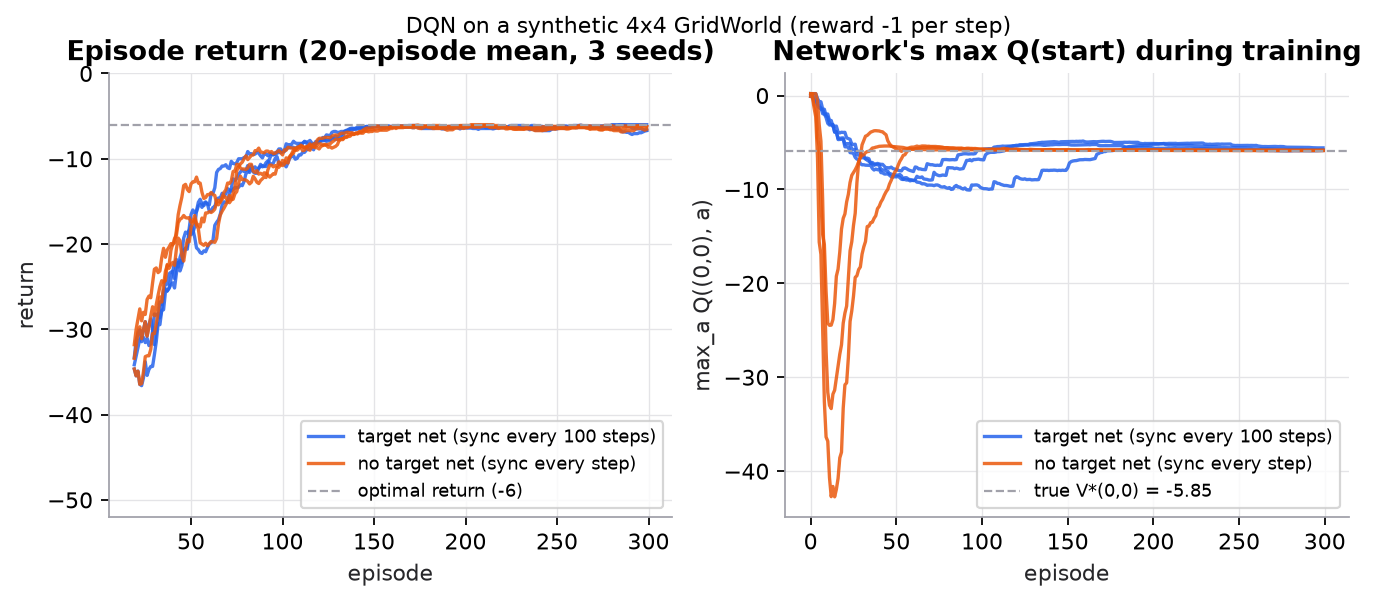
Synthetic environment: 4×4 GridWorld, start (0,0), goal (3,3), reward −1 per step, . Both variants use replay; orange copies the weights into the target every step, which is the same as having no target network. Produced by code/26-reinforcement-learning/dqn.py.
On this tiny problem both variants learn the optimal 6-step path. The difference is in the right panel. The true value of the start state is . With a target network the estimate drifts smoothly toward it. Without one, the estimate overshoots to in one seed, seven times too pessimistic, because every update shifts the label it is being fit to. One-hot states make this net almost a table, so it recovers. With pixels and shared features, the same feedback loop is what made naive deep Q-learning diverge.
Try it (predict first, then run the script and check):
- Change
sync_every=100tosync_every=1000. Predict whether learning gets faster or slower, and why a target that is too stale also hurts. - Set
warmup=32andcapacity=32so the buffer only holds the latest transitions. Predict what happens to the Q(start) curve when replay can no longer decorrelate data. - Set
eps_decay_eps=10so exploration collapses after 10 episodes. Predict whether the agent still finds the goal on every seed. - Replace the Huber gradient with the raw TD error (
g = delta). Predict which panel changes most early in training, when TD errors are large.
3. The math
Symbols
| Symbol | Meaning | Shape / type |
|---|---|---|
| state, action, reward, next state of one transition | state vector here, action index, scalar, | |
| 1 if is terminal, else 0 | scalar | |
| online network's Q-values for all actions | (one per action) | |
| online network weights (trained every step) | 676 numbers here | |
| target network weights (copied from every steps) | same as | |
| discount factor | scalar in | |
| replay buffer of recent transitions | up to 2,000 tuples here | |
| TD target (the regression label) | scalar | |
| TD error | scalar | |
| exploration probability | scalar in |
The network here is : parameters.
The DQN loss
The target uses the frozen network and does not bootstrap past a terminal state:
The loss averages a penalty on the TD error over a minibatch sampled uniformly from the buffer:
Gradients flow only through , never through . In a framework you enforce this with no_grad or detach on the target computation.
is usually the Huber loss with threshold :
It is squared error near zero and absolute error far away, so a single surprising transition cannot produce a huge gradient. The 2015 DQN paper got the same effect by clipping the error term to .
Double DQN (van Hasselt et al., 2016) changes only the target. The online network picks the next action and the target network scores it:
Taking a max over noisy estimates is biased upward: if four actions are all truly worth and each estimate has noise, the largest of the four estimates is usually above . Using two networks to select and evaluate means one network's lucky noise is not also the one that scores it.
Worked example: one transition
Transition , , , . Mid-training estimates (hand-picked, close to the true values):
- Target network at , actions (up, down, left, right):
- Online network at :
- Online
- Best target-network value at : (down).
- TD target: .
- TD error: .
- , so Huber is quadratic: .
- Gradient with respect to : . Gradient descent lowers from toward . The other three outputs get zero gradient.
- Compare a large error, : Huber with gradient 1; squared error with gradient 3. Huber caps the step at a third of the size.
- Double DQN target: the online network's best action at is right ( is the largest of its four values). The target network scores right as . So .
The Double DQN target is lower, less optimistic, because it did not take the target network's own maximum. For reference, the true optimal value of is .
4. Implementation
The full script is code/26-reinforcement-learning/dqn.py (NumPy only). It builds DQN in four pieces, prints the worked example above, then trains with and without a target network.
Build it from scratch
Step 1: the environment and the state encoding. A 4×4 grid, start top-left, goal bottom-right, per step so shorter paths score higher. Moving into a wall leaves you in place. The network cannot read a tuple, so each state becomes a one-hot vector of length 16.
def step(s, a):
    r, c = s
    dr, dc = DELTAS[a]
    nxt = (min(max(r + dr, 0), GRID - 1), min(max(c + dc, 0), GRID - 1))  # walls: stay put
    return nxt, -1.0, nxt == GOAL

def features(s):  # one-hot state, shape [16]
    x = np.zeros(GRID * GRID)
    x[s[0] * GRID + s[1]] = 1.0
    return x
Predict: with one-hot inputs, does an update for state (0,0) change the Q-values of state (0,1)? (Look at which weights are shared in step 2.)
Step 2: the Q-network. Linear, ReLU, linear. One forward pass returns all four action values at once, which is why DQN suits small discrete action sets: the greedy action is one argmax.
def init_net(rng, n_in=16, n_hidden=32, n_out=4):
    return {"W1": rng.normal(0, 0.3, (n_in, n_hidden)), "b1": np.zeros(n_hidden),
            "W2": rng.normal(0, 0.3, (n_hidden, n_out)), "b2": np.zeros(n_out)}

def forward(net, X):  # X: [B, 16] -> Q: [B, 4], hidden: [B, 32]
    H = np.maximum(0.0, X @ net["W1"] + net["b1"])
    return H @ net["W2"] + net["b2"], H
Predict: how would you change this network for an action space of 10,000 discrete actions? For a continuous steering angle?
Step 3: the Huber TD loss and one gradient step. The target comes from target, the online network is the only one updated, and the (1.0 - D) factor stops bootstrapping at the goal. Backprop is written out by hand: only the column for the action actually taken gets a gradient.
def huber(delta, k=1.0):
    """Quadratic for |delta| <= k, linear beyond: the gradient is clipped to [-k, k]."""
    a = np.abs(delta)
    return np.where(a <= k, 0.5 * delta**2, k * (a - 0.5 * k)), np.clip(delta, -k, k)

def train_step(online, target, batch, gamma, lr):
    S, A, R, S2, D = batch                                     # shapes [B,16], [B], [B], [B,16], [B]
    q_next, _ = forward(target, S2)                            # frozen network builds the target
    y = R + gamma * (1.0 - D) * q_next.max(axis=1)             # no bootstrap past a terminal state
    Q, H = forward(online, S)
    idx = np.arange(len(A))
    loss, g = huber(Q[idx, A] - y)                             # g = dLoss/dQ(s,a), clipped
    dQ = np.zeros_like(Q)
    dQ[idx, A] = g / len(A)                                    # only the taken action gets gradient
    dH = (dQ @ online["W2"].T) * (H > 0)
    grads = {"W2": H.T @ dQ, "b2": dQ.sum(0), "W1": S.T @ dH, "b1": dH.sum(0)}
    for k in online:
        online[k] -= lr * grads[k]
    return loss.mean()
Predict: what changes if you delete (1.0 - D)? Which state's value is wrong first, and in which direction? To make this Double DQN, which single line changes?
Step 4: the outer loop: replay, epsilon decay, target sync. Act epsilon-greedily, store every transition, and once the buffer has warmup transitions train on a uniform random minibatch each step. Every sync_every environment steps, copy the online weights into the target.
    for ep in range(episodes):
        eps = max(eps_end, 1.0 - ep / eps_decay_eps)           # linear decay 1.0 -> 0.05
        s, total = (0, 0), 0.0
        for _ in range(max_steps):
            if rng.random() < eps:
                a = int(rng.integers(4))
            else:
                a = int(forward(online, features(s)[None])[0][0].argmax())
            s2, r, done = step(s, a)
            buffer.append((features(s), a, r, features(s2), float(done)))
            total += r
            if len(buffer) >= warmup:
                picks = rng.choice(len(buffer), batch, replace=False)   # uniform, decorrelated
                S, A, R, S2, D = zip(*(buffer[i] for i in picks))
                train_step(online, target, (np.array(S), np.array(A), np.array(R), np.array(S2), np.array(D)), gamma, lr)
            steps += 1
            if steps % sync_every == 0:
                target = {k: v.copy() for k, v in online.items()}      # hard copy theta -> theta^-
            s = s2
            if done:
                break
The buffer is a deque(maxlen=capacity), so the oldest transitions fall off automatically. Predict: the agent stores transitions collected under an old, more random policy and still learns from them. Why is that allowed for Q-learning but not for the REINFORCE algorithm in the next lesson?
Use the library
In practice you use PyTorch through a library. Stable-Baselines3 (needs torch, gymnasium, and stable-baselines3; not run here) maps one keyword to each piece you just built:
import gymnasium as gym
from stable_baselines3 import DQN

env = gym.make("CartPole-v1")
model = DQN(
    "MlpPolicy", env,
    learning_rate=1e-3,
    buffer_size=50_000,          # replay capacity
    learning_starts=1_000,       # warmup before the first gradient step
    batch_size=32,
    gamma=0.99,
    target_update_interval=500,  # C: hard copy of theta into theta^- every 500 steps
    exploration_fraction=0.1,    # decay epsilon over the first 10% of training ...
    exploration_final_eps=0.05,  # ... down to 0.05
    train_freq=4,                # one gradient step every 4 environment steps
    seed=0,
)
model.learn(total_timesteps=50_000)
What the library adds: autograd instead of hand-written backprop, Adam instead of plain SGD, gradient-norm clipping, vectorized environments, and logging. SB3's DQN is the vanilla algorithm with the Huber (smooth L1) loss; Double DQN is a one-line change to the target, and single-file implementations such as CleanRL's are good to read next to this lesson. Frame stacking and reward clipping for Atari come from environment wrappers, not from the algorithm.
Run it
uv run code/26-reinforcement-learning/dqn.pyKey output (from guide/):
DQN target   y = -1 + 0.99 * max[-5.6, -4.9, -5.8, -5.0] = -5.851
TD error     delta = Q(s,a) - y = -5.2 - (-5.851) = 0.651
Huber loss   0.5 * delta^2 = 0.2119, gradient = 0.651
if delta = 3: Huber = 2.5 (grad 1), MSE 0.5*delta^2 = 4.5 (grad 3)
Double DQN   online picks right, target scores it -5.0 -> y = -5.950

=== DQN, target net (sync every 100 steps), 300 episodes, seeds [0, 1, 2] ===
mean return, last 50 episodes: -6.32   (optimal -6)
max Q(0,0) at the end per seed: [-5.57, -5.8, -5.84]   (true V*(0,0) = -5.852)
lowest max Q(0,0) during training per seed: [-10.1, -9.0, -8.1]

=== DQN, no target net (sync every step), 300 episodes, seeds [0, 1, 2] ===
mean return, last 50 episodes: -6.37   (optimal -6)
lowest max Q(0,0) during training per seed: [-42.7, -33.3, -24.5]
The first five lines reproduce the worked example. The last-50 mean is slightly below because stays at 0.05, so about one action in twenty is random.
5. Engineering
When DQN fits. Discrete, small action sets (game controls, a handful of routing or recommendation choices) with a simulator or plenty of logged transitions. Because it is off-policy and replays old data, it is sample-efficient compared with on-policy methods. For continuous actions use an actor-critic such as SAC or TD3, which keep the replay buffer and target networks but add a policy network. For LLM fine-tuning, the action space is the whole vocabulary at every token, and practice uses policy-gradient methods (PPO, GRPO) rather than Q-learning.
The improvements that stuck. Rainbow (Hessel et al., 2018) combined six extensions and reported that they add up:
- Double DQN: separate action selection from evaluation in the target (section 3). Cheap, and a sensible default.
- Dueling architecture: the network outputs a state value and per-action advantages , combined as . Helps when many actions have similar value.
- Prioritized experience replay: sample transitions with large TD error more often, and correct the resulting bias with importance-sampling weights.
- n-step returns, distributional Q (C51, QR-DQN), and noisy networks for learned exploration.
Hyperparameters that matter. The 2015 Atari DQN used a 1M-transition buffer, minibatch 32, target sync every 10,000 steps, decayed from 1.0 to 0.1 over the first million frames, rewards clipped to , and 4 stacked frames as the state so velocity is visible. Treat these as a starting point for Atari-like problems, not universal values.
Compute and memory. The buffer often dominates memory. One 84×84 grayscale frame is 7,056 bytes. Storing a 4-frame state and next state per transition would be bytes, about 56 GB for a million transitions; storing each frame once and indexing into it brings that to about 7 GB.
Watch outFailure modes. Divergence or oscillating Q-values (check the target sync and learning rate); overestimation, with Q-values far above any achievable return (use Double DQN); policy collapse after epsilon hits its floor too early; a non-Markov state (single frames with no velocity); and reward scales so large that gradients explode.
Common mistakes
- Letting gradients flow through the target . It must be computed with the target network and treated as a constant.
- Bootstrapping past a terminal state (forgetting ), or treating a time-limit cutoff as terminal. A truncated episode is not a real end, so you should still bootstrap there.
- Training on the first few transitions before the buffer has a reasonable warmup.
- Syncing the target every step (no stabilization) or so rarely that targets are stale.
- Decaying to zero, or decaying it before the agent has ever reached the reward.
- Judging progress by the training loss. A falling TD loss can mean the network agrees with its own wrong targets; watch episode return on evaluation runs with .
6. Knowledge check
Quiz: Deep Q-networks (DQN)
A non-terminal transition has and . The target network's Q-values at are . What is the DQN target ?
Practice exercise. A transition goes from to a terminal goal state with , . The target network's values at are . The online network's . Compute the TD target, the TD error, the Huber loss, and its gradient. Then do the same for a non-terminal version of the transition.
Solution
Terminal: , so . . , so Huber and the gradient is : the update raises .
Non-terminal: . . Huber , gradient . Squared error would give with gradient , more than six times larger.
Implementation challenge. Add Double DQN to dqn.py: in train_step, choose the next action with the online network and evaluate it with the target network. Then add Gaussian noise () to every reward and compare the final of DQN and Double DQN against the true value over 5 seeds.
Solution sketch
Replace the target line with:
q_next_online, _ = forward(online, S2)
a_star = q_next_online.argmax(axis=1)
y = R + gamma * (1.0 - D) * q_next[np.arange(len(A)), a_star]
With noisy rewards the vanilla max picks whichever action got lucky noise, so its Q(start) tends to sit above (optimistic). Double DQN's estimate should be closer, often slightly below. Report the mean and spread over seeds rather than a single run, since five seeds of a toy problem is a small sample.
Summary
- DQN is Q-learning with a neural network: outputs one value per action, trained by regression toward the TD target.
- Experience replay breaks the correlation between consecutive transitions and reuses data; it works because Q-learning is off-policy.
- The target network freezes the regression label between syncs; without it the label moves with every step and estimates can swing wildly or diverge.
- Huber loss caps the gradient at 1, so rare large TD errors cannot dominate an update. Epsilon decays from 1 to a small floor.
- Double DQN uses the online net to select and the target net to evaluate, reducing max-operator overestimation; dueling heads and prioritized replay are other standard upgrades.
- DQN suits small discrete action sets; continuous control uses SAC or TD3, and LLM fine-tuning uses policy gradients.
Next: Policy gradients and REINFORCE
Related: Q-learning and SARSA · PPO · Backpropagation · Training and regularization
Parts of this lesson are adapted from AI Engineering from Scratch by Rohit Ghumare (MIT license, notice): Deep Q-Networks (DQN).
Interview angle
What problems do experience replay and the target network each solve in DQN?
They fix two different instabilities. Experience replay fixes the data: transitions arrive as a stream where consecutive samples are nearly identical and the distribution shifts as the policy changes. SGD assumes roughly independent samples, so DQN stores recent transitions in a buffer and trains on uniform random minibatches. That decorrelates the batch and lets each transition be reused many times, which improves sample efficiency. It is only valid because Q-learning is off-policy: the target uses a max, not the behaviour policy's action. The target network fixes the label. The TD target uses Q of the next state, so with one network every gradient step moves the target too, and the regression can chase itself into oscillation or divergence. A frozen copy, synced every C steps or softly averaged, holds the target still long enough to fit it.
When would you pick DQN over PPO, and when the other way round?
DQN suits small discrete action spaces where samples are expensive. It is off-policy, so it can learn from a replay buffer of old transitions and even from logged data, and it often needs fewer environment steps. Its weaknesses: the greedy action needs a max over actions, which breaks down for continuous or huge action spaces; bootstrapped targets plus function approximation can be unstable; and it tends to need more tuning. PPO is on-policy, so it throws data away after a few epochs and needs more samples, but it is stable, handles continuous actions and very large discrete spaces (it only samples from a policy distribution), and scales well with many parallel simulators. Cheap simulator or continuous control: PPO or SAC. Atari-like discrete control with a costly simulator: DQN variants such as Rainbow. LLM fine-tuning: policy gradients, since the action space is the vocabulary.
Your DQN's predicted Q-values keep climbing far above any return the agent can actually achieve. What is happening and what do you check?
That is overestimation, and the usual source is the max in the target. With noisy estimates, the max over actions picks whichever action got positive noise, so the target is biased upward; bootstrapping then feeds that inflated value into earlier states and the error compounds. First I check the setup: is the target network actually used, and is its sync interval reasonable? Are terminal states masked, so the agent is not bootstrapping past the end? Is the learning rate too high, are rewards scaled sensibly, and is the loss Huber? Then I switch to Double DQN, where the online network selects the next action and the target network evaluates it, which removes most of the bias. I monitor mean predicted Q against actual discounted returns from evaluation episodes; they should track each other.
Size the replay buffer for an Atari DQN with 1 million transitions of 4 stacked 84×84 grayscale frames.
One frame is 84 × 84 = 7,056 bytes as uint8. A state is 4 frames, 28,224 bytes, and a transition needs both the state and the next state, so a naive buffer stores 56,448 bytes per transition. Times one million is about 56 GB, which is too much for most single machines. But consecutive states share 3 of their 4 frames, and the next state shares 3 frames with the current one. So real implementations store each frame once in a circular array, plus the action, reward, and done flag, and rebuild stacks by index at sampling time. That is about 7,056 bytes per transition, roughly 7 GB for a million. Further savings come from compression, a smaller buffer, or storing observations on disk. Always use uint8, never float32, which would multiply everything by four.