Module 25: Computer vision and multimodal 40 min9 min quick readDeep learning
Semantic segmentation and U-Net
Label every pixel with a class, explain why U-Net pairs an encoder and decoder with skip connections, combine cross-entropy with Dice loss for imbalanced masks, and report per-class IoU.
Before this: Convolutional networks, Object detection and YOLO
Quick read: the intuition, interactive visualization, summary, and interview questions. The math, implementation, engineering, and knowledge-check sections are hidden.
Mental model. Segmentation is classification run once per pixel. The hard part is that each pixel's label needs two kinds of knowledge at once: what the scene is (which needs a wide view) and exactly where the edge is (which needs full resolution). U-Net gets both by shrinking the image to understand it, growing it back to draw the answer, and passing the fine detail across the middle like notes from the way down.
You will learn to
- Distinguish semantic, instance, and panoptic segmentation and pick the right one for a task.
- Trace tensor shapes through a U-Net encoder, bottleneck, and decoder with skip connections.
- Compute per-class IoU and Dice by hand, and convert between them.
- Explain why pixel accuracy and plain cross-entropy fail on imbalanced masks, and how Dice loss fixes it.
- Diagnose a segmentation model from per-class metrics.
Why it matters. Tumour masks, road and lane maps for driving, building footprints from satellites, crop boundaries, defect regions on a production line: none of these can be solved with a box. They need the exact outline. U-Net (2015) is still the default starting point for medical and industrial segmentation, and its encoder-decoder-with-skips shape reappears in diffusion models.
1. Intuition
For an image of height and width , a segmentation model outputs a label for each of the pixels. A 512 by 512 image means 262,144 predictions, not one.
Three variants of the task:
- Semantic segmentation: every pixel gets a class ("road", "car", "sky"). Two touching cars merge into one "car" blob.
- Instance segmentation: every object gets its own mask ("car #3", "car #5"). Usually only countable "things", not background "stuff" like sky.
- Panoptic segmentation: both. Every pixel gets a class, and every thing gets an instance id.
This lesson covers semantic segmentation. Instance segmentation typically adds a mask head to a detector (object detection).
Why a plain classifier backbone is not enough. A CNN classifier halves the resolution several times to gain context: by the last layer, a 256 by 256 image is an 8 by 8 grid of very informative but very blurry features. Upsampling that grid back to 256 by 256 gives blocky, smeared edges. Small objects may vanish entirely.
U-Net's answer. Build a mirror image:
- Encoder (left side of the "U"): convolution blocks, each followed by max-pooling. Resolution halves, channels double.
- Bottleneck: the smallest, most semantic feature map.
- Decoder (right side): upsample by 2, then convolution blocks. Resolution doubles, channels halve.
- Skip connections: at each resolution, concatenate the encoder's feature map onto the decoder's. The decoder now sees both "this region is a tumour" (from below) and "the edge is exactly here" (from across).
- A final convolution maps each pixel's features to class scores.
Imbalance. In a medical scan, 99 percent of pixels can be background. A model that predicts "background" everywhere is 99 percent accurate and useless. That is why segmentation is scored with IoU per class and trained with overlap-based losses like Dice.
2. Visualization
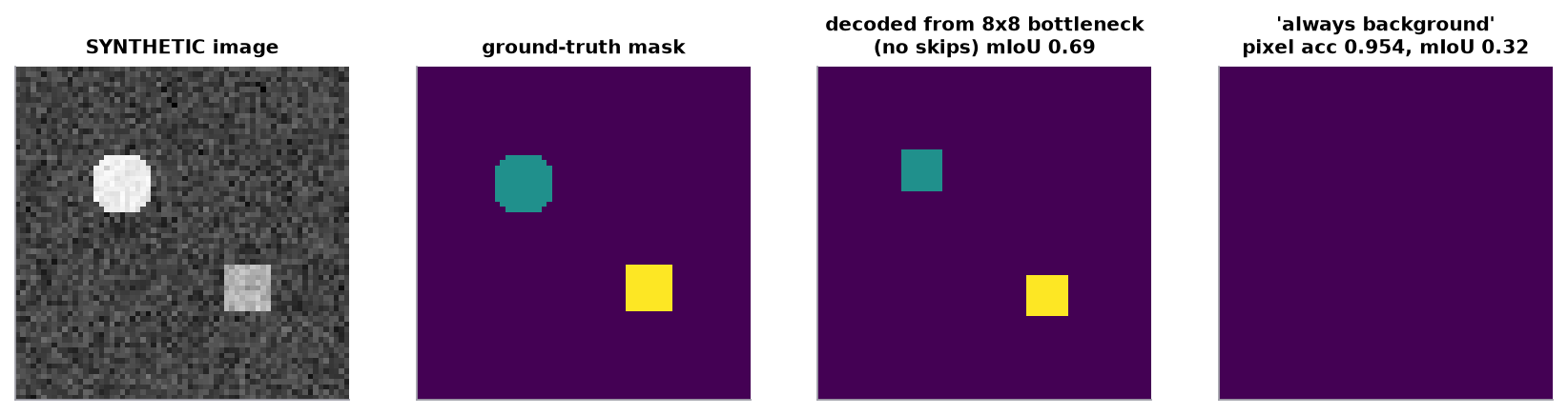
Synthetic scene: two small objects cover under 5 percent of the pixels. Decoding from a coarse bottleneck alone loses the shapes; predicting all background looks 95 percent accurate but finds nothing.
Try it (predict first, then check with the script in section 4):
- The script decodes from bottlenecks of 32, 16, 8, and 4 pixels per side. Predict roughly where mean IoU collapses, then run it.
- Shrink the circle radius from 6 to 3 pixels. Which bottleneck size now loses it completely?
- Compute the "always background" pixel accuracy for a scene where objects cover 20 percent of pixels. Is pixel accuracy now a better metric?
- In the transposed-convolution check, try kernel 6 with stride 4. Will the overlap pattern be even?
3. The math
Symbols
| Symbol | Meaning | Shape |
|---|---|---|
| image height and width | scalars | |
| number of classes | scalar | |
| logits from the model | ||
| softmax probabilities per pixel | ||
| ground-truth class id per pixel | ||
| sets of pixels predicted as / truly in class | sets | |
| small constant to avoid division by zero | scalar |
Pixel cross-entropy
Exactly classification cross-entropy, averaged over pixels. Every pixel counts equally, so the background dominates.
IoU and Dice per class
mIoU is the mean of over classes present in the image or dataset. Dice is the pixel version of the F1 score.
Soft Dice loss
Replace the hard sets with probabilities so the loss is differentiable:
Each class contributes equally no matter how many pixels it covers. The usual recipe is with : cross-entropy gives smooth gradients early, Dice keeps the small classes from being ignored.
Shapes through a U-Net
Input , base width 64. Each encoder level halves the size and doubles channels:
| Level | Encoder output | Decoder input after concat | Decoder output |
|---|---|---|---|
| 0 | |||
| 1 | |||
| 2 | |||
| 3 | |||
| bottleneck |
The final convolution gives . Four halvings mean the input side must be divisible by . With bilinear upsampling (no learned upsampling weights) this network has 31.4 million parameters at base 64 and 7.8 million at base 32 (the script counts them).
Worked example: IoU, Dice, and accuracy on a 4 by 4 mask
Ground truth: a 2 by 2 object in the middle. Prediction: three of those pixels plus one wrong pixel to the right.
truth        prediction
0 0 0 0      0 0 0 0
0 1 1 0      0 1 1 1
0 1 1 0      0 1 0 0
0 0 0 0 0 0 0 0- Foreground counts: , , .
- Union: . IoU .
- Dice . Check: .
- Pixel accuracy: 2 pixels wrong out of 16, so .
Pixel accuracy looks good because 12 of the 16 pixels are easy background. IoU shows that the object itself is only 60 percent right.
Worked example: the imbalance trap
In the synthetic scene above, background covers 95.36 percent of pixels, the circle 2.66 percent, the square 1.98 percent. Predict background everywhere:
- Pixel accuracy .
- IoU: background (prediction covers everything, truth covers 95.36 percent), circle , square .
- mIoU .
Soft losses on the same scene (from the script): confident logits that always say "background" get cross-entropy 0.2215, close to the 0.0360 of a confident correct model. Their soft Dice loss is 0.667, far from the correct model's 0.200. Dice sees the failure; cross-entropy barely does.
4. Implementation
The full script is code/25-computer-vision/segmentation_scratch.py (NumPy only). It implements the losses and metrics, the imbalance trap, a "no skip connections" experiment, the U-Net parameter count, and the transposed-convolution overlap check.
Build it from scratch
Step 1: pixel cross-entropy. The fancy indexing picks, at every pixel, the probability of that pixel's true class. Nothing else changes from classification.
def pixel_cross_entropy(logits, target):
    """logits: [C, H, W]; target: [H, W] integer class ids. Mean over pixels."""
    p = softmax(logits, axis=0)
    h, w = target.shape
    p_true = p[target, np.arange(h)[:, None], np.arange(w)[None, :]]   # prob of the true class at each pixel
    return float(-np.log(p_true + 1e-12).mean())
Predict: the logits are all zero (an untrained model). With 3 classes, what loss should this return? (The script prints it.)
Step 2: soft Dice loss. One-hot the target, then compute overlap over total per class and average. Because each class is a ratio of its own pixels, a 2 percent class weighs as much as a 95 percent one.
def soft_dice_loss(logits, target, eps=1e-6):
    """1 - mean over classes of 2|P∩Y| / (|P| + |Y|), with P = softmax probabilities."""
    c = logits.shape[0]
    p = softmax(logits, axis=0)
    y = np.eye(c)[target].transpose(2, 0, 1)            # one-hot [C, H, W]
    inter = (p * y).sum(axis=(1, 2))
    denom = p.sum(axis=(1, 2)) + y.sum(axis=(1, 2))
    return float(1 - ((2 * inter + eps) / (denom + eps)).mean())
Predict: a class is absent from both the target and the prediction in this batch. With eps, what Dice score does that class get, and is that what you want when averaging?
Step 3: per-class IoU. Return nan for a class that appears in neither mask, so np.nanmean skips it instead of counting a meaningless 0 or 1.
def iou_per_class(pred, target, c):
    out = []
    for k in range(c):
        inter = np.sum((pred == k) & (target == k))
        union = np.sum((pred == k) | (target == k))
        out.append(inter / union if union else np.nan)    # nan = class absent from both: skip it in the mean
    return np.array(out)
Predict: for the "always background" prediction, why is the background IoU exactly equal to the background pixel fraction?
Step 4: what a decoder without skips can recover. Simulate the information left at the bottleneck: average the one-hot mask over blocks, take the majority class, and blow it back up. Real decoders do better than nearest-neighbour upsampling, but they cannot recover detail that was averaged away.
def down_up(mask, factor, c):
    """Squeeze the mask through a bottleneck of size/factor (majority vote per block), then blow it back up.
    This is what a decoder WITHOUT skip connections has to work with."""
    s = mask.shape[0] // factor
    onehot = np.eye(c)[mask].reshape(s, factor, s, factor, c).mean(axis=(1, 3))   # [s, s, C] class fractions
    coarse = onehot.argmax(-1)
    return np.repeat(np.repeat(coarse, factor, 0), factor, 1)
Predict: at a factor of 16, each block is 16 by 16 = 256 pixels. Can a 12-pixel-wide circle ever win a majority vote in such a block?
Step 5: count U-Net parameters. Each "double conv" is two convolutions without bias, each followed by batch norm (2 learned numbers per channel). Decoder blocks take the upsampled channels plus the skip channels.
def double_conv(cin, cout):            # conv3x3 (no bias) + BN + ReLU, twice
    return cin * cout * 9 + 2 * cout + cout * cout * 9 + 2 * cout

def unet_params(base=64, cin=3, classes=2):
    ch = [base, base * 2, base * 4, base * 8, base * 16]
    n = double_conv(cin, ch[0]) + sum(double_conv(ch[i], ch[i + 1]) for i in range(4))   # encoder + bottleneck
    for i in range(4, 0, -1):                                   # decoder: concat skip, then DoubleConv
        n += double_conv(ch[i] + ch[i - 1], ch[i - 1])
    return n + base * classes + classes                         # final 1x1 conv
Predict: halving base from 64 to 32 divides the parameter count by roughly what factor? (Most weights are cin * cout products.)
Use the library
In PyTorch the same pieces are a few lines; segmentation_models_pytorch (smp) builds a U-Net on any pretrained encoder.
import torch.nn.functional as F
import segmentation_models_pytorch as smp                  # pip install segmentation-models-pytorch

model = smp.Unet(encoder_name="resnet34", encoder_weights="imagenet", in_channels=3, classes=3)
logits = model(images)                                       # [N, 3, H, W], H and W divisible by 32
ce = F.cross_entropy(logits, masks)                          # masks: [N, H, W] int64; no reshaping needed
dice = smp.losses.DiceLoss(mode="multiclass")(logits, masks)
loss = ce + dice
What the library adds: an ImageNet-pretrained encoder (far better than training from scratch on a few hundred masks), batch norm and ReLU wiring, handling of odd sizes, and other architectures behind the same API (DeepLabV3+, FPN, and transformer encoders). For transformer segmenters (SegFormer, Mask2Former) see Hugging Face transformers. For promptable masks (click a point, get the object), the Segment Anything family is the 2025-era default.
Run it
uv run code/25-computer-vision/segmentation_scratch.pyKey lines of output (the scene is synthetic):
class pixel fractions (background, circle, square): [0.9536, 0.0266, 0.0198]
pixel accuracy = 0.9536
IoU per class  = [0.9536, 0.0, 0.0]  -> mIoU 0.3179
IoU fg = 0.6000, Dice fg = 0.7500, check 2*IoU/(1+IoU) = 0.7500
always background      CE = 0.2215   soft Dice loss = 0.6670
bottleneck 1/8  (8x8): mIoU after upsampling = 0.6904
bottleneck 1/16 (4x4): mIoU after upsampling = 0.3179
params base=64: 31,384,898   base=32: 7,849,634
kernel 3, stride 2: contributions per output pixel = [1, 2, 1, 2, 1, 2, 1, 2, 1, 2, 1]
kernel 4, stride 2: contributions per output pixel = [2, 2, 2, 2, 2, 2, 2, 2, 2, 2]
The last two lines explain checkerboard artifacts: with kernel 3 and stride 2, alternate output pixels receive one or two contributions, which shows up as a grid pattern. Kernel 4 (divisible by the stride) or bilinear upsampling plus a convolution avoids it.
5. Engineering
Use cases. Medical imaging (organs, tumours, lesions), autonomous driving (drivable area, lanes), remote sensing (buildings, fields, water), document layout, industrial defect masks, photo editing (background removal).
Labels are the bottleneck. Pixel masks take minutes per image. Options: start from a pretrained encoder, use interactive tools (promptable segmenters) to draft masks and have people correct them, label coarse polygons first, and measure inter-annotator IoU so you know the ceiling.
Resolution and memory. Activations scale with channels. A 1024 by 1024 input to a base-64 U-Net already takes gigabytes for activations during training. Standard workarounds: train on random crops and predict with overlapping tiles stitched together, use mixed precision, or use dilated convolutions (DeepLab) to keep resolution without huge maps.
Metrics to report. Per-class IoU or Dice, plus mIoU. Add a boundary metric (boundary F1) when edge accuracy matters, such as in semiconductor inspection or surgical planning. Medical work tends to report Dice; driving benchmarks report IoU; they rank models the same way because Dice is a monotonic function of IoU.
Post-processing. Remove tiny connected components, fill holes, and enforce known topology (one liver per scan). Calibrate a per-class threshold on validation data instead of always taking the argmax when one class is much rarer.
Watch outFailure modes. Small, thin structures (vessels, cracks) vanish at coarse resolution; class imbalance makes the model predict background; boundaries blur when only the bottleneck is upsampled; resizing masks with bilinear interpolation creates invalid in-between class ids (always use nearest-neighbour for masks); domain shift (a new scanner, a new city) breaks texture cues the encoder learned.
Common mistakes
- Reporting pixel accuracy on imbalanced data.
- Reporting only mIoU, hiding a rare class at 0.3 among others at 0.9.
- Interpolating label masks with anything other than nearest-neighbour.
- Feeding input sizes not divisible by and silently cropping or misaligning skip connections.
- Averaging IoU over batches where a class is absent as if it scored 0.
- Augmenting the image (flip, rotate, crop) without applying the identical transform to the mask.
6. Knowledge check
Quiz: Semantic segmentation and U-Net
Why does U-Net need skip connections between encoder and decoder?
Practice exercise. A model predicts 60 tumour pixels. The ground truth has 50 tumour pixels, and 40 pixels are in both. Compute IoU and Dice for the tumour class. If the image has 10,000 pixels and everything else is correct, what is the pixel accuracy?
Solution
Union , so IoU . Dice . Check: . Wrong pixels: 20 false positives () and 10 false negatives (), 30 in total. Pixel accuracy . Pixel accuracy says 99.7 percent; the tumour mask is only 57 percent right by IoU.
Implementation challenge. Add a binary focal term to the script: with , where is the probability of the true class. Compare its value with plain cross-entropy for the "always background" logits. Which loss penalises the missed objects more, relative to how it scores the easy background pixels?
Solution sketch
def pixel_focal(logits, target, gamma=2.0):
    p = softmax(logits, axis=0)
    h, w = target.shape
    pt = p[target, np.arange(h)[:, None], np.arange(w)[None, :]]
    return float((-(1 - pt) ** gamma * np.log(pt + 1e-12)).mean())
For the always-background logits, background pixels have , so shrinks their loss by about 800 times, while object pixels have and keep almost all of theirs. The total loss becomes dominated by the missed objects, which is exactly what focal loss is for.
Summary
- Semantic segmentation predicts a class per pixel; instance segmentation separates objects; panoptic does both.
- U-Net shrinks the image for context, grows it back for resolution, and concatenates encoder features into the decoder at every level so edges survive.
- Pixel cross-entropy treats every pixel equally and gets dominated by background; Dice loss scores each class by overlap, so combine them.
- Report per-class IoU or Dice (Dice = 2 IoU / (1 + IoU)), never pixel accuracy alone.
- Pretrained encoders, crops and tiling, and nearest-neighbour mask resizing are the practical defaults.
Next: Vision transformers
Related: Object detection and YOLO · Convolutional networks · Classification metrics · Autoencoders, diffusion, and transfer
Go deeper, code-first (AI Engineering from Scratch): SAM 3 & Open-Vocabulary Segmentation
Parts of this lesson are adapted from AI Engineering from Scratch by Rohit Ghumare (MIT license, notice): Semantic Segmentation — U-Net.
Interview angle
Why does U-Net need skip connections? What would happen without them?
The encoder trades resolution for context: after four poolings a 256-pixel image is a 16 by 16 grid whose features know what is in each region but not where its edges are within that region. A decoder that only upsamples this bottleneck has to invent the detail. Edges come out blocky, and objects smaller than a bottleneck cell can disappear. In the synthetic example here, squeezing the mask through an 8 by 8 grid drops mean IoU from 1.0 to 0.69, and a 4 by 4 grid erases both small objects. Skip connections concatenate the encoder's high-resolution feature map at each level into the decoder at the same level. The decoder then combines "this region is a tumour" from below with "the boundary is exactly here" from across. They also shorten gradient paths, which helps training, much as residual connections do.
Cross-entropy versus Dice loss: when would you use each, and why combine them?
Pixel cross-entropy treats every pixel equally, so a class covering 2 percent of pixels contributes about 2 percent of the loss. Its gradients are smooth and well behaved, especially early in training. Dice loss scores each class by the ratio of overlap to total size, so a tiny tumour counts as much as the background. It directly targets the overlap metric you report, but it is noisy when a class has very few pixels in a batch, and its gradients can be unstable early on. In the synthetic scene here, confident "all background" logits get cross-entropy 0.22, close to a perfect model's 0.04, but soft Dice loss 0.67 versus 0.20. The common recipe is cross-entropy plus Dice with equal weight: cross-entropy for stable optimisation, Dice to stop rare classes from being ignored. Focal loss and class weights are alternatives.
Your segmentation model reports mIoU 0.78 but clinicians say it misses small lesions. How do you investigate?
First break the mean apart: per-class IoU, and within the lesion class, IoU or recall by lesion size. A mean of 0.78 is consistent with large organs at 0.9 and small lesions at 0.3. Compute lesion-level detection recall (did any predicted pixel overlap each lesion?) as well as pixel IoU, since one large lesion can dominate pixel metrics. Then check where small lesions are lost. Inspect resolution: if inputs were downsampled to fit memory, small lesions may be only a few pixels. Check the loss: plain cross-entropy under-weights rare pixels, so add Dice or focal loss. Check post-processing, since removing small connected components deletes exactly these lesions. Finally check labels: small lesions are often inconsistently annotated. Fixes include higher-resolution tiles, size-aware sampling, a lower per-class threshold, and reporting metrics stratified by lesion size.
Quick calculation: a 1024 by 1024 input goes through a four-level U-Net with base width 64. What are the bottleneck shape and the largest activation?
Four poolings divide each side by 16, so the bottleneck is 1024 / 16 = 64 pixels per side with 64 × 2⁴ = 1024 channels: a 1024 × 64 × 64 tensor, about 4.2 million values. The largest activations are actually at full resolution: the first double convolution outputs 64 × 1024 × 1024 ≈ 67 million values, and the last decoder level concatenates 128 + 64 = 192 channels at 1024 by 1024, about 201 million values. In fp32 that single concatenated tensor is about 805 MB, and training stores many such activations per image for the backward pass. That is why high-resolution segmentation trains on crops (say 256 or 512 pixels), uses mixed precision, and predicts on overlapping tiles stitched back together. The input side must also be divisible by 16.