Module 25: Computer vision and multimodal 40 min12 min quick readDeep learning
Self-supervised vision
Learn visual features without labels using contrastive learning (SimCLR), self-distillation (DINO), and masked reconstruction (MAE); compute the InfoNCE loss by hand; and evaluate features with linear probes.
Before this: Vision transformers, Learning paradigms
Quick read: the intuition, interactive visualization, summary, and interview questions. The math, implementation, engineering, and knowledge-check sections are hidden.
Mental model. Labels are expensive, but images carry their own homework. Show a network two different crops of the same photo and ask it to recognise they belong together; or hide three quarters of the photo and ask it to paint the rest back in. To pass these made-up tests it has to learn what objects look like. Afterwards you throw the test away and keep the knowledge.
You will learn to
- Explain the three families of self-supervised vision: contrastive (SimCLR, MoCo), self-distillation (BYOL, DINO), and masked image modelling (MAE, BEiT).
- Compute the InfoNCE (NT-Xent) loss for a small batch by hand, and predict how temperature and batch size change it.
- Explain what representation collapse is and how negatives, centring, sharpening, or reconstruction prevent it.
- Explain why MAE masks 75 percent of patches while BERT masks 15 percent of tokens.
- Evaluate a pretrained encoder with a linear probe and k-nearest-neighbour retrieval.
Why it matters. A labelled dataset like ImageNet took years of crowd work; unlabelled images are nearly free. Self-supervised pretraining lets you learn from the unlabelled pile and then fine-tune on a few thousand labelled examples. Self-supervised backbones (DINOv2 and successors, MAE) are the default general-purpose visual features in 2026, and the contrastive loss here is the same one CLIP uses for images and text (next lesson).
1. Intuition
In self-supervised learning the data provides its own targets through a pretext task. The pretext task does not matter in itself. It is useful only if solving it forces the network to learn features that transfer, such as shapes, parts, and object identity.
Three families have scaled well.
1. Contrastive (SimCLR, MoCo). Take a batch of images. Make two random views of each: random crop, flip, colour jitter, blur. Encode all views. For each view, its twin is the positive; the other views are negatives. Train so each view is closer to its twin than to any negative. To succeed, the encoder must ignore what the augmentations change (colour, crop position) and keep what they preserve (it's a dog). More negatives make the task harder and the signal sharper, so SimCLR used batches of 4,096 or more. MoCo keeps a queue of recent embeddings from a slowly updated momentum encoder, which decouples the number of negatives from batch size.
2. Self-distillation (BYOL, DINO). No negatives at all. A student network sees one view and must predict the output of a teacher network that sees another view. The teacher is not trained by gradients: its weights are an exponential moving average (EMA) of the student's. The obvious cheat is collapse: output the same vector for every image and the student matches the teacher perfectly. DINO prevents this with two tricks on the teacher's output: centring (subtract a running mean, so no single dimension can win for every image) and sharpening (a low softmax temperature, so the output can't drift to uniform). Centring alone pushes toward uniform; sharpening alone pushes toward one dimension. Together they balance.
3. Masked image modelling (MAE, BEiT). Cut the image into patches as in a ViT, hide most of them, and reconstruct the hidden ones. MAE hides 75 percent. Images are highly redundant: with only 15 percent hidden, the network could fill each gap by blurring its neighbours, without understanding anything. At 75 percent it has to know what objects look like. MAE's encoder sees only the visible 25 percent, which makes pretraining cheap; a small decoder fills in the rest and is discarded after pretraining.
How do we know the features are good? Freeze the encoder and train only a linear classifier on top: a linear probe. If a straight line separates the classes in feature space, the encoder already did the hard work. A k-nearest-neighbour classifier on frozen features is an even simpler check. Fine-tuning the whole network gives higher numbers but mixes in the effect of further training.
NoteThe families have different strengths. Contrastive and self-distillation methods produce features that work well frozen (good linear probes, retrieval). MAE features tend to need fine-tuning to shine but scale cheaply and suit dense tasks. DINOv2 combines self-distillation with a masked-patch objective (from iBOT) on a large curated dataset, which is why it is a common frozen backbone for retrieval, depth, and segmentation.
2. Visualization
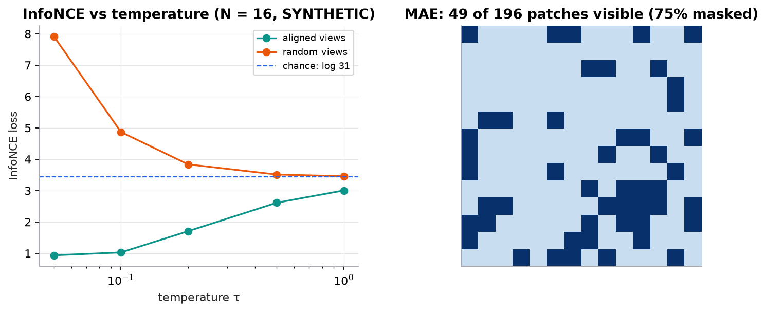
Lower temperature rewards well-aligned views and punishes unrelated ones much harder. MAE keeps 49 of 196 patches visible.
Try it (predict first, then check with the script in section 4):
- Random views at score 4.39, above the chance level of 3.43. Predict why "random" can be worse than "uniform guessing".
- Double the batch from 16 to 32 pairs. What happens to the chance-level loss, and what does that say about comparing loss values across batch sizes?
- In the DINO demo, set the sharpening temperature to 0.5 instead of 0.04. Predict the entropy compared with 0.101 (sharp) and 2.768 (no sharpening).
- Change the MAE ratio to 0.5. How much more attention compute does the encoder spend?
3. The math
Symbols
| Symbol | Meaning | Shape |
|---|---|---|
| images per batch (giving views) | scalar | |
| L2-normalised embedding of view | ||
| cosine similarity, for unit vectors | scalar | |
| temperature | scalar | |
| index of view 's twin | ||
| student and teacher weights | ||
| EMA momentum (DINO uses about 0.996 rising to 1) | scalar | |
| MAE mask ratio | scalar |
InfoNCE (NT-Xent), as in SimCLR
It is cross-entropy where the "classes" are the other views and the correct class is the twin. If the softmax were uniform, every view would score : that is the chance level.
DINO teacher update and output
The student minimises the cross-entropy between on one view and its own on another. is small (0.04 to 0.07), larger (0.1).
MAE
The mean squared error over masked patches only; . The encoder processes patches, so its attention cost falls by about : 16 times for .
Worked example: InfoNCE with N = 2
Two images, so four views, all already unit length, :
- image A: ,
- image B: ,
Cosines (dot products): , , , , , .
View (twin ). Candidates: with logits , , .
- Exponentials: , , . Sum .
- Probability on the twin: .
- .
View (twin ). Candidates: with logits , , .
- Exponentials: , , . Sum .
- Probability on the twin: .
- .
By symmetry and . The loss is , below the chance level .
View is the hard one: its closest neighbour is (cosine 0.96), a negative. The gradient pushes and apart and pulls toward . Hard negatives like this carry most of the learning signal, which is why more negatives help.
4. Implementation
The full script is code/25-computer-vision/ssl_scratch.py (NumPy only). It implements InfoNCE, reproduces the worked example, sweeps temperature and batch size, builds an MAE mask, and shows DINO's collapse and its fix.
Build it from scratch
Step 1: InfoNCE. Stack both views into one matrix, compute all pairwise cosines at once, mask the diagonal (a view is not its own candidate), and run cross-entropy where the target for row is its twin rows away.
def info_nce(z1, z2, tau=0.1):
    """z1, z2: [N, D] unit vectors; row i of z1 and row i of z2 are two views of image i."""
    n = len(z1)
    z = np.concatenate([z1, z2])                      # [2N, D]
    sim = z @ z.T / tau                               # [2N, 2N] cosine / temperature
    np.fill_diagonal(sim, -np.inf)                    # a view is never its own candidate
    target = np.concatenate([np.arange(n, 2 * n), np.arange(n)])   # view i's twin sits N rows away
    return float(-log_softmax(sim)[np.arange(2 * n), target].mean())
Predict: if you forgot fill_diagonal, each row's largest logit would be its self-similarity . With identical views, what would the loss approach as ?
Step 2: MAE masking. A random permutation, keep the first 25 percent. Sorting keeps the visible patches in grid order, which makes adding position embeddings straightforward.
def random_mask(num_patches, ratio=0.75, seed=0):
    perm = np.random.default_rng(seed).permutation(num_patches)
    keep = int(num_patches * (1 - ratio))
    return np.sort(perm[:keep]), np.sort(perm[keep:])
Predict: MAE adds position embeddings to the visible patches before dropping the masked ones. Why must positions be attached before the encoder, rather than after?
Step 3: DINO's teacher output. Subtract the centre, divide by a temperature, softmax. The demo gives every sample a shared offset in one dimension to mimic the start of collapse, then measures how many distinct "winning" dimensions remain and how peaked each output is.
def teacher_probs(logits, centre, temp):
    return np.exp(log_softmax((logits - centre) / temp))

def collapse_report(p):
    entropy = -(p * np.log(p + 1e-12)).sum(-1).mean()
    return len(set(p.argmax(-1))), entropy
Predict: with centring but a very high temperature (10), every output is close to uniform. Why is a uniform target also a form of collapse for the student?
Use the library
Pretrained self-supervised encoders are a download away. Use them frozen for retrieval and probes, or fine-tune.
import torch
from transformers import AutoImageProcessor, AutoModel       # pip install transformers torch pillow

proc = AutoImageProcessor.from_pretrained("facebook/dinov2-base")
model = AutoModel.from_pretrained("facebook/dinov2-base").eval()
with torch.no_grad():
    out = model(**proc(images=pil_images, return_tensors="pt"))
feats = torch.nn.functional.normalize(out.last_hidden_state[:, 0], dim=-1)   # [B, 768] CLS features

# linear probe: freeze feats, fit any linear classifier
from sklearn.linear_model import LogisticRegression
probe = LogisticRegression(max_iter=2000).fit(train_feats, train_labels)
What the libraries add: the augmentation pipelines (multi-crop for DINO), distributed negatives or queues, EMA teachers, the masking and decoder for MAE, and, most importantly, weights pretrained on far more images than you could process yourself. timm hosts MAE and DINO checkpoints; lightly packages SimCLR, MoCo, BYOL, and DINO training loops.
Run it
uv run code/25-computer-vision/ssl_scratch.pyKey lines of output (synthetic embeddings):
InfoNCE = 0.8707
identical views: 0.0073
random views:    4.3862   (chance level log(2N - 1) = log 31 = 3.4340)
tau 0.05: aligned 0.9355   random 7.9128
tau 1.0 : aligned 3.0036   random 3.4590
batch N = 4096: 8190 negatives, chance-level loss log(2N - 1) = 9.011
196 patches -> encoder sees 49, decoder reconstructs 147; first visible: [0, 5, 6, 10, 13, 35]
encoder self-attention scores: full 38,809 vs visible-only 2,500 (15.5x fewer)
no centring, sharp (temp 0.04)       distinct argmax =  1 / 16, mean entropy = 0.000 (uniform = 2.773)
centring, no sharpening (temp 10)    distinct argmax = 16 / 16, mean entropy = 2.768 (uniform = 2.773)
centring + sharpening (temp 0.04)    distinct argmax = 16 / 16, mean entropy = 0.101 (uniform = 2.773)
Random views score above chance at low temperature because their logits are spread out: the twin is often far from the top, and a confident wrong softmax costs more than a uniform one.
5. Engineering
When to pretrain yourself. Rarely from scratch. Start from a public self-supervised checkpoint. Continue self-supervised pretraining on your own unlabelled images when your domain looks unlike web photos (medical scans, satellite tiles, microscopy, industrial cameras), then fine-tune or probe with your labels.
Augmentations define the invariances. Contrastive and self-distillation methods learn to ignore whatever the augmentations change. Colour jitter teaches colour invariance, which is wrong if colour is the label (ripe versus unripe fruit, some lesions). Choose augmentations per domain.
Compute. Contrastive methods need many negatives: large batches across GPUs or a memory queue. DINO needs several crops per image (two global, several local). MAE is the cheapest per step because the encoder sees a quarter of the patches; pretraining throughput is several times higher than encoding every patch.
Evaluation. Report a linear probe and k-NN accuracy on frozen features, plus fine-tuned accuracy on the target task. Use a held-out labelled set that was never used to pick augmentations or checkpoints.
Watch outFailure modes. Collapse (all embeddings identical: watch the per-dimension standard deviation of the embeddings, which falls toward zero); shortcut learning (views from the same image share a colour histogram or a JPEG artefact the network can match without understanding content); batch-norm information leaking between views in contrastive training (MoCo used shuffling BN to prevent it); false negatives (two different photos of the same product treated as negatives).
Common mistakes
- Comparing InfoNCE values across batch sizes. The chance level is , so a bigger batch has a bigger loss for the same quality.
- Judging a self-supervised model by its pretext loss instead of a downstream probe.
- Copying ImageNet augmentation settings to a domain where colour or orientation is meaningful.
- Using MAE features frozen and concluding they are weak; they usually need fine-tuning.
- Forgetting to normalise embeddings before the dot product, so the "cosine" is unbounded.
6. Knowledge check
Quiz: Self-supervised vision
Why did SimCLR need very large batches (thousands of images)?
Practice exercise. A batch has images. How many negatives does each view have in SimCLR? What InfoNCE loss would a model that outputs uniform probabilities get? If a model assigns probability 0.25 to the twin on average, roughly what is its loss?
Solution
views. Each view has 1 positive and negatives. Uniform probabilities over the 255 candidates give . Probability 0.25 on the twin gives per view, about 1.39 on average (exactly, if every view assigns 0.25).
Implementation challenge. Implement the BYOL / DINO EMA teacher update for a weight dictionary and measure how fast the teacher follows the student: set student weights to all ones, teacher to zeros, and apply 100 updates with and then . What fraction of the gap is closed?
Solution sketch
def ema(teacher, student, m):
    return {k: m * teacher[k] + (1 - m) * student[k] for k in teacher}

t, s = {"w": np.zeros(3)}, {"w": np.ones(3)}
for _ in range(100):
    t = ema(t, s, 0.99)
print(t["w"][0])   # 1 - 0.99**100 = 0.634
After updates the teacher has closed of the gap: 63.4 percent at , and percent at . A higher momentum gives a slower, more stable teacher, which is why DINO raises toward 1 during training.
Summary
- Self-supervised learning makes its own targets: match two views (contrastive), match an EMA teacher (self-distillation), or reconstruct hidden patches (masked image modelling).
- InfoNCE is cross-entropy over candidates; temperature sets how hard it punishes near misses, and more negatives give a sharper signal.
- Collapse is the central risk; negatives, centring plus sharpening, or a reconstruction target prevent it.
- MAE masks 75 percent because images are redundant, and it encodes only visible patches, which makes it cheap.
- Judge features by linear probe, k-NN, and fine-tuning on held-out labels, never by the pretext loss.
Next: CLIP and contrastive image-text pretraining
Related: Vision transformers · Learning paradigms · Word embeddings · Autoencoders, diffusion, and transfer
Parts of this lesson are adapted from AI Engineering from Scratch by Rohit Ghumare (MIT license, notice): Self-Supervised Vision — SimCLR, DINO, MAE.
Interview angle
Explain the InfoNCE loss used by SimCLR. Why does batch size matter so much?
Each image in a batch of N gets two augmented views, giving 2N embeddings, all L2-normalised. For each view, compute its cosine similarity with the other 2N − 1 views, divide by a temperature τ, and apply softmax cross-entropy where the correct class is its twin. So the model plays a (2N − 1)-way matching game. Batch size matters because the other views in the batch are the negatives. With N = 32 each view has 62 negatives; with N = 4096 it has 8190. More negatives mean more hard negatives, look-alike images the encoder must separate, and a tighter estimate of the contrastive objective. That is why SimCLR trained with very large batches. MoCo avoids the memory cost with a queue of embeddings from a slowly updated momentum encoder, giving tens of thousands of negatives with ordinary batches. Remember that the chance-level loss, log(2N − 1), grows with batch size.
DINO uses no negatives. Why doesn't it collapse to a constant output?
Without negatives, the trivial solution is for student and teacher to output the same vector for every image, which gives zero loss. DINO prevents that with two operations on the teacher's output. Centring subtracts a running mean of teacher logits, so no single dimension can dominate across all images; on its own this pushes outputs toward uniform. Sharpening uses a low teacher temperature, around 0.04, so each output is peaked; on its own that pushes toward one dominant dimension. The two pressures balance. In the synthetic demo here, sharpening without centring sends all 64 samples to the same dimension, centring without sharpening gives near-uniform outputs, and both together give 16 distinct winners with low entropy. The EMA teacher also helps, because it changes slowly and gives the student a stable, slightly better target, and multi-crop views force local-to-global consistency.
Why does MAE mask 75 percent of patches when BERT masks 15 percent of tokens?
The right mask ratio depends on how much information each unit carries. Words are dense: a masked word in a sentence has many plausible completions, so even 15 percent masking is a hard prediction task. Image patches are redundant: neighbouring patches are strongly correlated, so with 15 percent masked the network could interpolate from surrounding pixels and learn little about objects. Masking 75 percent removes most of the local context, so reconstruction requires knowing what things look like. High masking also makes MAE efficient. The encoder only processes visible patches, 49 of 196 at 224 pixels, so attention per layer drops from about 38,800 scores to 2,500 per head. A lightweight decoder handles the mask tokens and is discarded after pretraining. Mask ratio is a hyperparameter, and very high ratios work best for images and video.
You pretrained a contrastive model on your factory images and the linear probe is barely above chance. What do you check?
First check for collapse. Compute the per-dimension standard deviation of normalised embeddings across a batch. If it is near zero, every image maps to the same point; check temperature, learning rate, and whether there are enough negatives. Second, check for shortcuts. If both views share a camera ID watermark, a timestamp, or a lighting signature, the network can match views without learning defects. Look at nearest neighbours: are they the same station rather than the same defect? Third, check the augmentations against the label. If defects are colour or fine-texture changes, strong colour jitter and blur teach the model to ignore exactly what you need. Fourth, check false negatives: near-identical parts from the same line are pushed apart. Finally, sanity-check the probe itself. Compare it with a public DINOv2 checkpoint on the same split. If the generic model wins, continue pretraining from it instead of from scratch.