Module 25: Computer vision and multimodal 35 min9 min quick readDeep learning
Vision transformers
Turn an image into a sequence of patch tokens, trace shapes through a ViT, count its parameters, explain how patch size sets cost, and choose between ViT, hierarchical transformers, and CNNs.
Before this: Convolutional networks, The transformer architecture
Quick read: the intuition, interactive visualization, summary, and interview questions. The math, implementation, engineering, and knowledge-check sections are hidden.
Mental model. Cut the photo into a grid of small square tiles, flatten each tile into a list of numbers, and treat each tile like a word. Then run the same transformer you would run on a sentence. Nothing in the model knows it is looking at an image, except that it learned where each tile came from.
You will learn to
- Convert an image into patch tokens and compute the token count for any image and patch size.
- Show that patch embedding is a single matrix multiply, equivalently a convolution with kernel size equal to stride.
- Trace tensor shapes through a ViT: patches, [CLS] token, position embeddings, encoder blocks, classifier.
- Count the parameters of ViT-B/16 and explain how patch size drives attention cost.
- Explain why ViTs needed large datasets or strong training recipes, and when to choose a CNN, ViT, or hierarchical transformer.
Why it matters. Since 2020, transformers have taken over most of vision: the image towers in CLIP and SigLIP, the encoders inside every vision-language model, segmentation (SegFormer, Mask2Former), detection (DETR family), and self-supervised backbones (DINOv2, MAE). If you know the ViT recipe, all of these are small variations.
1. Intuition
A transformer takes a sequence of vectors and lets every vector look at every other one through self-attention. To use it on an image, we need a sequence.
Pixels as tokens do not work. A 224 by 224 image has 50,176 pixels. Attention compares every pair, so that would be about 2.5 billion pairs per head per layer. Far too many.
Patches as tokens do. Cut the image into 16 by 16 tiles. A 224-pixel side gives tiles per side, so tiles. Each tile holds numbers. A learned linear layer maps each flattened tile to a -dimensional token. Now we have 196 tokens, like a 196-word sentence.
Three more pieces finish the ViT:
- A [CLS] token. One extra learned vector placed at the front. After the transformer layers, its output summarises the whole image, and the classifier reads only that one vector. (Many recent models average all patch outputs instead.)
- Position embeddings. Attention has no notion of order or layout. A learned vector is added to each token according to its grid position, so the model can tell the top-left tile from the bottom-right.
- Encoder blocks. The standard pre-norm transformer block: layer norm, multi-head self-attention, residual add; layer norm, MLP, residual add. ViT-B stacks 12 of them.
What changes compared with a CNN. A CNN builds in two assumptions: nearby pixels matter most (locality), and a cat is a cat wherever it appears (translation equivariance). A ViT builds in neither. From the first layer, any patch can attend to any other patch. That flexibility is why it scales so well, and also why it needs more data or more augmentation to learn what a CNN gets for free. The original ViT (2020) lost to ResNets when trained on ImageNet-1k alone but won after pretraining on a 300-million-image dataset. DeiT (2021) closed the gap on ImageNet-1k with heavy augmentation, regularisation, and distillation. Self-supervised pretraining (next lesson) is now the other common fix.
2. Visualization
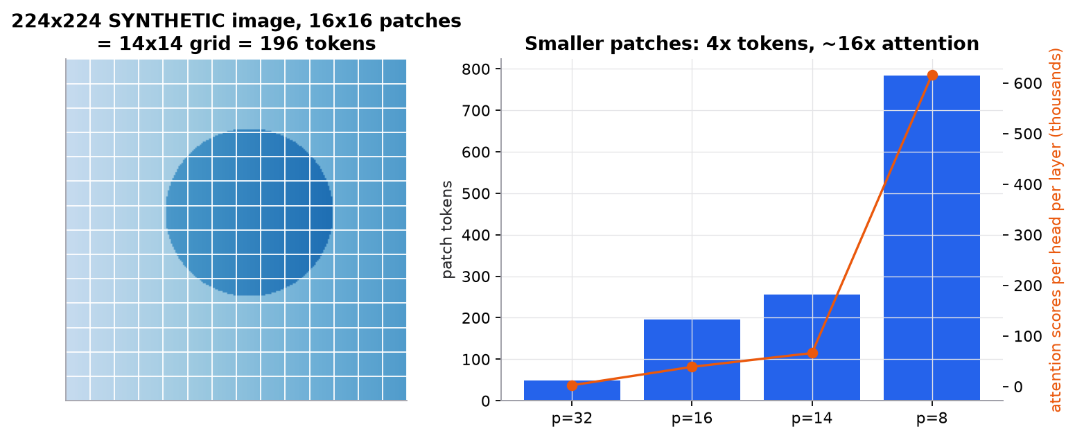
Halving the patch size quadruples the tokens and multiplies the attention matrix by about 16. Patch size is the main knob trading detail against compute.
Try it (predict first, then check with the script in section 4):
- A 384 by 384 image with 16 by 16 patches: how many tokens? How many attention scores per head per layer, counting [CLS]?
- Predict ViT-B/16's parameter count if you drop the classifier head (1000 classes). Which part of the model holds most of the parameters?
- In the tiny ViT, change the patch size from 8 to 4. What are the new shapes of
patchesandtok? - You fine-tune at 384 pixels a model pretrained at 224. The learned position table has 197 rows but you now have 577 tokens. What would you do?
3. The math
Symbols
| Symbol | Meaning | Shape |
|---|---|---|
| image height, width, channels | scalars | |
| patch side in pixels | scalar | |
| number of patches, | scalar | |
| flattened patches | ||
| patch embedding matrix | ||
| learned [CLS] vector | ||
| learned position embeddings | ||
| model width | scalar | |
| number of encoder blocks | scalar |
Forward pass
is row 0 of the final output, the [CLS] token. The MLP is with GELU.
Patch embedding is a convolution
Multiplying each flattened patch by is the same as a convolution with filters of size and stride : each filter visits each patch exactly once and computes the same dot product. Libraries implement it as Conv2d(C, D, kernel_size=P, stride=P).
Worked example: ViT-B/16 shapes and parameters
, , , , , 12 heads, 1000 classes.
- Patches: . Each patch has values. is .
- Tokens after embedding, [CLS], and positions: . Each head works in dimensions.
- Patch embedding parameters: .
- [CLS] and position embeddings: .
- One encoder block:
- two layer norms:
- Q, K, V projections:
- attention output projection:
- MLP up:
- MLP down:
- total:
- Twelve blocks: .
- Final layer norm and head .
- Total: , the familiar "86M".
Almost 98 percent of the parameters sit in the encoder blocks, and two thirds of each block is the MLP.
Patch size and cost
Attention compares every token with every token: scores per head per layer. At 224 pixels:
| Patch | Grid | Tokens | Scores |
|---|---|---|---|
| 32 | 7 × 7 | 49 | 2,500 |
| 16 | 14 × 14 | 196 | 38,809 |
| 14 | 16 × 16 | 256 | 66,049 |
| 8 | 28 × 28 | 784 | 616,225 |
Halving multiplies by 4 and attention cost by about 16. Doubling image resolution at fixed has the same effect. This quadratic growth is why hierarchical models like Swin compute attention inside local windows, which makes cost linear in the number of patches.
4. Implementation
The full script is code/25-computer-vision/vit_scratch.py (NumPy only). It patchifies a synthetic image, embeds the patches, proves the embedding equals a strided convolution, runs one encoder block, and reproduces the parameter and cost tables above.
Build it from scratch
Step 1: patchify. Reshape so each axis splits into (which patch, position inside the patch), move the two patch-grid axes to the front, then flatten. No loops, no copies of pixels beyond the final reshape.
def patchify(img, p):
    """img: [H, W, C] -> [N, p*p*C] with N = (H/p) * (W/p), patches in row-major order."""
    h, w, c = img.shape
    assert h % p == 0 and w % p == 0, "image size must be divisible by the patch size"
    x = img.reshape(h // p, p, w // p, p, c)        # split both spatial axes into (grid, within-patch)
    x = x.transpose(0, 2, 1, 3, 4)                  # [gh, gw, p, p, C]: group pixels by patch
    return x.reshape(-1, p * p * c)
Predict: if you skipped the transpose, the shapes would still work. What would each "patch" row actually contain?
Step 2: patch embedding equals a strided convolution. Embedding is patches @ W_e. The loop version below slides a filter bank with stride ; the script checks the two agree to floating-point precision.
def conv_patch_embed(img, kernel, p):
    """The same thing as a conv with kernel = stride = p (no padding). kernel: [D, p, p, C]."""
    h, w, _ = img.shape
    out = []
    for i in range(0, h, p):
        for j in range(0, w, p):
            out.append(np.tensordot(kernel, img[i:i + p, j:j + p], axes=([1, 2, 3], [0, 1, 2])))
    return np.array(out)
Predict: what changes if the stride is smaller than the patch size, say kernel 16 and stride 8? How many tokens would a 224-pixel image give?
Step 3: one pre-norm encoder block. Layer norm goes inside each residual branch, so the residual stream itself is never normalised. That is what lets deep stacks train without careful warmup. Heads are a reshape: [n, d] becomes [heads, n, d/heads].
def encoder_block(x, P, heads):
    n, d = x.shape
    dh = d // heads
    h = layer_norm(x)                                                   # pre-LN: normalise the input of the sublayer
    q, k, v = ((h @ P[w]).reshape(n, heads, dh).transpose(1, 0, 2) for w in ("Wq", "Wk", "Wv"))
    a = softmax(q @ k.transpose(0, 2, 1) / np.sqrt(dh))                 # [heads, n, n]: every patch sees every patch
    x = x + (a @ v).transpose(1, 0, 2).reshape(n, d) @ P["Wo"]          # residual 1
    x = x + gelu(layer_norm(x) @ P["W1"]) @ P["W2"]                     # residual 2: MLP d -> 4d -> d
    return x, a
Predict: the attention map a has shape [heads, 17, 17] in the tiny model. Which row would you inspect to see which patches the [CLS] token attends to?
Step 4: assemble and count. Prepend [CLS], add positions, run the blocks, read row 0. The parameter counter mirrors the worked example line by line.
def vit_params(d=768, depth=12, p=16, img=224, c=3, classes=1000, mlp=4):
    n = (img // p) ** 2
    patch = p * p * c * d + d
    tokens = d + (n + 1) * d                                           # [CLS] + position embeddings
    block = 2 * 2 * d + (d * 3 * d + 3 * d) + (d * d + d) + (d * mlp * d + mlp * d) + (mlp * d * d + d)
    return patch + tokens + depth * block + 2 * d + d * classes + classes, block
Predict: ViT-L/16 uses and 24 blocks. Roughly how many parameters, using "about per block"?
Use the library
timm provides every common ViT variant with pretrained weights. Hugging Face transformers provides the same, plus the CLIP, SigLIP, and DINOv2 vision towers.
import timm, torch                                            # pip install timm torch

model = timm.create_model("vit_base_patch16_224", pretrained=True, num_classes=10)  # new 10-class head
print(model.patch_embed.proj)        # Conv2d(3, 768, kernel_size=(16, 16), stride=(16, 16))
logits = model(torch.randn(2, 3, 224, 224))                   # [2, 10]

# fine-tune at a new resolution: timm interpolates the position embeddings for you
model384 = timm.create_model("vit_base_patch16_224", pretrained=True, img_size=384)
What the library adds: the conv patch embedding, fused attention kernels, dropout and stochastic depth, pretrained weights from large datasets, and 2-D interpolation of the position table when you change resolution (the answer to "Try it" question 4).
Run it
uv run code/25-computer-vision/vit_scratch.pyKey lines of output (random weights, synthetic image):
image (32, 32, 3) -> patches (16, 192) -> tokens (16, 16)
matmul patch embedding == conv(kernel=stride=8): True
with [CLS] and position embeddings: (17, 16)
after one encoder block: (17, 16); attention maps (2, 17, 17); rows sum to 1: True
one encoder block: 7,087,872
total (224x224, 1000 classes): 86,567,656
patch 16: 14x14 =  196 patch tokens,    38,809 attention scores per head per layer
patch  8: 28x28 =  784 patch tokens,   616,225 attention scores per head per layer
5. Engineering
Choosing a backbone.
| Situation | Reasonable default |
|---|---|
| Small labelled dataset, fine-tune | Pretrained ViT or ConvNeXt; both work, pick what your stack supports |
| Dense prediction (segmentation, detection) at high resolution | Hierarchical backbone (Swin, ConvNeXt) or a ViT with windowed attention |
| Edge device, tight latency | Efficient CNN (MobileNet family, small ConvNeXt), or a distilled small ViT if the runtime supports attention well |
| Image-text tasks, vision-language models | CLIP or SigLIP ViT towers (CLIP lesson) |
| General-purpose frozen features | Self-supervised ViT (DINOv2 family) |
ConvNeXt (2022) showed that a CNN modernised with transformer-era design and training choices matches Swin. The gap was mostly recipe, not attention versus convolution.
Training recipe. From scratch on a mid-sized dataset, a ViT needs strong augmentation (RandAugment, Mixup, CutMix), regularisation (stochastic depth, weight decay), and long schedules. In practice, almost everyone fine-tunes a pretrained checkpoint instead.
Resolution. Fine-tuning at a higher resolution than pretraining usually helps, but it changes the token count. Interpolate the position embeddings in 2-D (not 1-D over the flattened sequence), and budget for the quadratic attention cost.
Throughput. Tokens, not parameters, set the cost. Token merging or pruning, larger patches, and FlashAttention-style kernels are the levers. ViT-B/16 at 224 pixels processes 197 tokens; the same model at 448 pixels processes 785.
Watch outFailure modes. Training a ViT from scratch on a few thousand images and concluding "transformers don't work here"; position-embedding size mismatches when loading a checkpoint at a new resolution; image sizes not divisible by the patch size, silently cropped; mismatched normalisation constants (ImageNet mean and std versus CLIP's) between pretraining and fine-tuning; attention maps over-interpreted as explanations.
Common mistakes
- Thinking ViT parameter count grows with image size. Only the position table does; compute grows quadratically.
- Forgetting the [CLS] token when counting sequence length (197, not 196).
- Using the ImageNet classifier's features for retrieval when a contrastive or self-supervised backbone would be far better.
- Comparing ViT and CNN results trained with different recipes and data, then attributing the gap to architecture.
- Resizing the position table with 1-D interpolation over the flattened sequence.
6. Knowledge check
Quiz: Vision transformers
How does a ViT turn an image into a sequence of tokens?
Practice exercise. A ViT-S/16 has , 12 blocks, 6 heads, MLP ratio 4. For a 224 by 224 input, compute: the number of tokens including [CLS], the dimension per head, and the parameters in one encoder block.
Solution
Tokens: . Per head: . One block: layer norms ; QKV ; output projection ; MLP up ; MLP down . Total , close to . Twelve blocks give about 21.3 million, so ViT-S is about 22M parameters with the embeddings and head.
Implementation challenge. Replace the [CLS] token with mean pooling: drop the extra token, run the block on the 16 patch tokens, and average the outputs. Then implement 2-D interpolation of a position table from a 4 by 4 grid to an 8 by 8 grid (bilinear, on the grid, not on the flattened list), and check the output shape.
Solution sketch
y, _ = encoder_block(tok + pos[1:], params, HEADS)      # no [CLS] row
pooled = y.mean(axis=0)                                  # [D]

def resize_pos(pos_grid, new):                           # pos_grid: [g, g, D]
    g = pos_grid.shape[0]
    xs = np.linspace(0, g - 1, new)
    i0 = np.floor(xs).astype(int); i1 = np.minimum(i0 + 1, g - 1); f = xs - i0
    rows = pos_grid[i0] * (1 - f)[:, None, None] + pos_grid[i1] * f[:, None, None]          # [new, g, D]
    return rows[:, i0] * (1 - f)[None, :, None] + rows[:, i1] * f[None, :, None]           # [new, new, D]
resize_pos(pos[1:].reshape(4, 4, D), 8).reshape(64, D) gives the 64 patch positions; keep the [CLS] position row unchanged if your model has one.
Summary
- A ViT cuts the image into patches, embeds each with one linear layer (a stride- convolution), adds a [CLS] token and learned positions, and runs a standard pre-norm transformer encoder.
- Token count is ; attention cost grows with its square, so patch size and resolution are the main compute knobs.
- ViT-B/16 has 86.6M parameters, almost all in its 12 encoder blocks; parameter count barely depends on resolution.
- ViTs have weaker built-in assumptions than CNNs, so they need large pretraining, strong augmentation, or self-supervision; with those, they are the default backbone for multimodal and general-purpose vision.
Next: Self-supervised vision
Related: Self-attention · The transformer architecture · Convolutional networks · CLIP
Go deeper, code-first (AI Engineering from Scratch): Video Understanding — Temporal Modeling · 3D Vision — Point Clouds & NeRFs
Parts of this lesson are adapted from AI Engineering from Scratch by Rohit Ghumare (MIT license, notice): Vision Transformers (ViT).
Interview angle
How does a ViT turn an image into tokens, and what does each piece of the input sequence do?
Split the image into non-overlapping P by P patches; at 224 pixels with P = 16 that is a 14 by 14 grid, 196 patches of 768 raw values each. Flatten each patch and multiply by a learned matrix to get a D-dimensional token. That is exactly a convolution with kernel size and stride both P, which is how libraries implement it. Prepend a learned [CLS] vector, giving 197 tokens; after the encoder, its output summarises the image and feeds the classifier (mean pooling over patch tokens is the common alternative). Add a learned position embedding to every token so the model knows each patch's location, because attention by itself is permutation-invariant. Then run L pre-norm transformer blocks, each multi-head self-attention plus an MLP with residual connections. Nothing image-specific happens after the patch embedding.
ViT versus CNN: what are the trade-offs, and when would you still pick a CNN?
A CNN builds in locality and translation equivariance, so it learns efficiently from modest data, and its cost grows linearly with pixel count. A ViT has global attention from layer one and almost no built-in assumptions, so it needs large pretraining, heavy augmentation, or self-supervision. Once it has that, it scales better with data and model size, and it plugs straight into multimodal stacks. Its cost grows quadratically with token count, which hurts at high resolution unless you use windowed attention as Swin does. ConvNeXt showed that much of the historical gap came from training recipe rather than architecture. I would still pick a CNN for edge deployment on runtimes where attention is poorly optimised, for very high-resolution dense prediction under tight memory, or for small from-scratch training. For anything feeding an LLM or needing general-purpose features, I would pick a pretrained ViT.
You fine-tune a ViT pretrained at 224 pixels on 384-pixel images and loading fails, or accuracy collapses. What is going on?
The learned position table has one row per token at pretraining resolution: 196 + 1 = 197 rows for a 14 by 14 grid. At 384 pixels with 16-pixel patches the grid is 24 by 24, giving 577 tokens. Loading fails with a shape mismatch if the code is strict. If it silently truncates or pads, patches get the wrong positions and accuracy collapses. The fix is to reshape the 196 patch positions into a 14 by 14 grid, interpolate in 2-D (bicubic or bilinear) to 24 by 24, flatten back, and keep the [CLS] row as is. timm does this when you pass img_size. Also check preprocessing: resize and crop settings, and normalisation constants, must match what the checkpoint expects. Finally, expect higher compute, because attention scores per layer grow from about 38,800 to about 333,000 per head.
Quick calculation: how many parameters does ViT-B/16 have, and where are they?
D is 768, there are 12 blocks, and the MLP is 4 times wider. Per block: Q, K, and V projections are 768 by 2304 plus bias, about 1.77M; the output projection is about 0.59M; the MLP is 768 by 3072 and back, about 4.72M; layer norms are negligible. That is about 7.09M per block, roughly 12 D², and 85.05M for 12 blocks. The patch embedding is 16 × 16 × 3 × 768 plus bias, about 0.59M. The [CLS] token and 197 position vectors add about 0.15M, and a 1000-class head about 0.77M. The total is about 86.6M. So 98 percent of the weights are in the encoder blocks and two thirds of each block is the MLP. Resolution barely changes parameters, only the position table, but it changes compute quadratically.