Module 13: Deep-learning architectures 35 min7 min quick readDeep learning
Autoencoders, diffusion, and transfer learning
Learn compressed representations with autoencoders, understand how diffusion models generate by reversing noise, and adapt pretrained models to new tasks with transfer learning.
Before this: The neural-network forward pass, Training and regularization, PCA, t-SNE, and UMAP
Quick read: the intuition, interactive visualization, summary, and interview questions. The math, implementation, engineering, and knowledge-check sections are hidden.
Mental model. An autoencoder squeezes data through a narrow bottleneck and learns to rebuild it, so the bottleneck must capture what matters. A diffusion model learns to undo noise one small step at a time, so starting from pure noise it can walk back to a realistic sample. Transfer learning reuses what a big model already learned instead of starting from zero.
You will learn to
- Describe the encoder, bottleneck, and decoder of an autoencoder, and its reconstruction loss.
- Explain latent spaces and uses such as denoising and anomaly detection.
- Explain diffusion's forward (noising) and reverse (denoising) processes and compute a noised sample.
- Apply transfer learning: feature extraction versus fine-tuning.
Why it matters. Representation learning underlies embeddings, anomaly detection, and generative models. Diffusion models generate most state-of-the-art images and audio. Transfer learning is how nearly every practical deep-learning project starts, including LLM fine-tuning.
1. Intuition
Autoencoders. Train a network to output its own input, with a deliberately narrow middle layer. It can't copy pixel by pixel, so it must learn a compact code, the latent representation. Uses: compression, denoising (train on noisy input, clean target), and anomaly detection (unusual inputs reconstruct poorly). A linear autoencoder with squared error learns the same subspace as PCA; nonlinear ones can capture curved structure.
Diffusion models. Take real data and add a little Gaussian noise, again and again, until nothing but noise remains (the forward process, fixed and easy). Train a network to predict the noise that was added at each step. To generate, start from random noise and repeatedly subtract the predicted noise (the reverse process). Conditioning on text lets you steer what gets generated.
Transfer learning. A model pretrained on a huge, broad dataset has learned general features (edges and textures for images; syntax and facts for language). For a new task, keep those features and train only a small new head (feature extraction), or continue training all or part of the model with a small learning rate (fine-tuning). This needs far less labeled data and compute.
2. Visualization
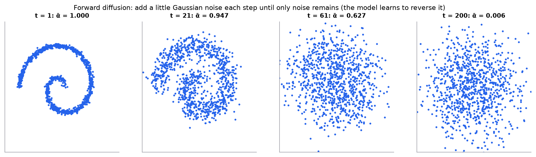
Synthetic spiral with a linear noise schedule over 200 steps. By the last step : almost none of the original signal remains. A diffusion model learns to run this movie backward.
3. The math
Symbols
| Symbol | Meaning |
|---|---|
| , | encoder and decoder |
| latent code (bottleneck) | |
| noise added at diffusion step (a small variance) | |
| fraction of signal variance remaining after steps | |
| standard Gaussian noise | |
| the network's prediction of the added noise |
Autoencoder
Variational autoencoders (VAEs) make the latent space probabilistic and smooth by adding a KL-divergence term, so you can sample new data from it.
Diffusion
Forward process in closed form (jump directly to any step):
Training objective (simplified DDPM loss): predict the noise.
Worked example: one noised sample
A data point at a step where , with sampled noise :
If the trained network predicts exactly, we can recover . Generation does this gradually, from pure noise, over many steps.
Worked example: transfer-learning parameter budget
A pretrained image backbone has 25 million parameters and outputs a 2,048-dimensional feature vector. A new 5-class head adds parameters. Feature extraction trains only those 10,245 (0.04% of the model), which is why it works with a few hundred labeled images.
4. Implementation
The full script is code/13-deep-architectures/generative_scratch.py (NumPy only, synthetic data). It trains an autoencoder by hand, shows the two extra pieces a VAE needs, and builds a complete one-dimensional diffusion model: schedule, forward noising, a trained noise predictor, and the reverse sampler.
Build it from scratch
Step 1: a linear autoencoder. Encode with E ([d, k]), decode with D ([k, d]), and run gradient descent on the squared reconstruction error. The two gradient lines are backpropagation through two matrix multiplies.
def train_autoencoder(X, k, lr=0.01, steps=3000):
    d = X.shape[1]
    E, D = rng.normal(scale=0.1, size=(d, k)), rng.normal(scale=0.1, size=(k, d))
    for _ in range(steps):
        Z = X @ E                                  # encode  [n, k]
        R = Z @ D - X                              # reconstruction error [n, d]
        gD = Z.T @ R / len(X)                      # dL/dD
        gE = X.T @ (R @ D.T) / len(X)              # dL/dE, chain rule through Z
        E, D = E - lr * gE, D - lr * gD
    return E, D
Predict: with no nonlinearity and a 2-number bottleneck, what is the best reconstruction this can reach? Compare it with PCA keeping 2 components.
Step 2: the VAE's two extra pieces. The encoder outputs a mean and a log-variance instead of one code. Sampling directly would block gradients, so write it as with the randomness moved into . The KL term, which pulls each code distribution toward , has a closed form.
def reparameterize(mu, log_var, eps):
    return mu + np.exp(0.5 * log_var) * eps        # z = mu + sigma * eps; randomness is in eps

def kl_to_standard_normal(mu, log_var):
    return 0.5 * np.sum(np.exp(log_var) + mu ** 2 - 1 - log_var)
Predict: for , in one dimension, the KL is . What is it, and what does the penalty push toward?
Step 3: the noise schedule and forward process. Pick a small for each step, compute as a running product, and jump to any step in one line with the closed-form formula from section 3.
T = 100
betas = np.linspace(1e-4, 0.2, T)                  # noise added at each step (larger than the
alphas = 1 - betas                                 # usual 0.02 because T is only 100)
alpha_bar = np.cumprod(alphas)                     # signal variance left after t steps

def noise(x0, t, eps):
    return np.sqrt(alpha_bar[t]) * x0 + np.sqrt(1 - alpha_bar[t]) * eps
Predict: is close to 0 or to 1? What does look like, whatever was?
Step 4: train the noise predictor. The DDPM loss is a regression: given , predict the that made it. Real models use a U-Net or transformer conditioned on . Here the data is one number, so a separate least-squares fit per step on five fixed features is enough, and it minimizes the same loss.
def fit_noise_predictor(n=4000):
    W = np.zeros((T, 5))
    for t in range(T):                             # minimize ||eps - eps_hat(x_t, t)||^2
        x0, eps = sample_data(n), rng.normal(size=n)
        W[t] = np.linalg.lstsq(features(noise(x0, t, eps)), eps, rcond=None)[0]
    return W
Predict: at small , is nearly . Is the noise easy or hard to predict there?
Step 5: generate. Start from pure noise. At each step, subtract the predicted noise (scaled for that step), rescale, and add a little fresh noise, except at the last step.
def sample(W, n):
    x = rng.normal(size=n)                         # x_T ~ N(0, 1)
    for t in reversed(range(T)):
        eps_hat = features(x) @ W[t]
        x = (x - betas[t] / np.sqrt(1 - alpha_bar[t]) * eps_hat) / np.sqrt(alphas[t])
        if t > 0:
            x += np.sqrt(betas[t]) * rng.normal(size=n)   # fresh noise, except at the last step
    return x
Predict: the data has two clusters, at and . Starting from a single Gaussian centered at 0, where do the samples end up?
Use the library
PyTorch supplies the networks and autograd; the Hugging Face diffusers library supplies production schedulers (DDPM, DDIM, and faster samplers that need tens of steps instead of hundreds) and pretrained U-Nets. For transfer learning, torchvision and timm supply pretrained backbones, so the only from-scratch part is the new head.
import torch
from torch import nn

# A small autoencoder for 28x28 images
autoencoder = nn.Sequential(
    nn.Flatten(), nn.Linear(784, 128), nn.ReLU(), nn.Linear(128, 16),   # encoder -> 16-d latent
    nn.ReLU(), nn.Linear(16, 128), nn.ReLU(), nn.Linear(128, 784), nn.Sigmoid(),
)
# loss = F.mse_loss(autoencoder(x), x.flatten(1))

# Transfer learning with torchvision: freeze the backbone, train a new head
from torchvision.models import resnet50, ResNet50_Weights
model = resnet50(weights=ResNet50_Weights.DEFAULT)
for p in model.parameters():
    p.requires_grad = False
model.fc = nn.Linear(model.fc.in_features, 5)      # only this layer trains at first
Run it
uv run code/13-deep-architectures/generative_scratch.pyKey lines of the output (all data is synthetic):
reconstruction MSE: autoencoder 0.00153, PCA 0.00151, data variance 0.937
z for eps = [0.5, -2]: [ 1.5 -1. ]
KL(N(mu, sigma^2) || N(0, 1)): 0.8181
x_t = 1.30;  recovered x0 = 2.00
t = 100: alpha_bar = 0.0000  (signal std 0.005)
fraction near -2: 0.51, near +2: 0.49, between (|x| < 1): 0.00
mean |x| = 1.99 (data: about 2.0)
A linear autoencoder reaches PCA's error, because the best linear 2-d code is the top-2 principal subspace. The fourth line is the worked example above. Starting from one Gaussian, the sampler splits the samples evenly between the two clusters and leaves none in the gap. The figure script is code/13-deep-architectures/architectures.py.
5. Engineering
Autoencoders for anomaly detection. Train on normal data only; flag inputs whose reconstruction error exceeds a threshold set on validation data. Watch out: a powerful autoencoder can reconstruct anomalies well too.
Diffusion in practice. Generation needs many network evaluations (tens to hundreds of steps), so it is expensive; distillation and faster samplers reduce steps. Latent diffusion runs the process in an autoencoder's latent space to cut cost. Evaluate generative models with human review and task-specific checks, not just automated scores.
Transfer learning choices.
| Situation | Approach |
|---|---|
| Little data, task similar to pretraining | freeze the backbone, train a head |
| Moderate data | fine-tune the top layers with a small learning rate |
| Lots of data, different domain | fine-tune everything, or pretrain on in-domain data |
Use a lower learning rate for pretrained layers than for the new head, and match the pretrained model's preprocessing (normalization, resolution, tokenizer). A common recipe is discriminative learning rates: the head at the base rate, and each earlier group of layers at a fraction of the one above it (for example 0.3×), because early layers hold generic edges and textures that need little change. When the fine-tuning batch is small, also freeze BatchNorm's running statistics (put those layers in eval mode); otherwise a few noisy batches overwrite statistics estimated on millions of images.
Watch outFailure modes. Catastrophic forgetting when fine-tuning too aggressively; preprocessing mismatches with the pretrained model; licensing restrictions on pretrained weights; generative models reproducing training data or harmful content; anomaly detectors that reconstruct anomalies too well.
Common mistakes
- Fine-tuning a large model with a large learning rate and destroying its features.
- Forgetting to put the frozen backbone in eval mode (batch-norm statistics drift).
- Treating reconstruction error as calibrated anomaly probability.
6. Knowledge check
Quiz: Autoencoders, diffusion, and transfer learning
With , , and , what is ? (3 decimals)
Practice exercise. With , , and , compute .
Solution
and : . At this step noise dominates the signal.
Implementation challenge. Train the small autoencoder on MNIST digits, plot reconstructions for latent sizes 2, 8, and 32, and use reconstruction error to flag a set of images that are not digits.
Summary
- Autoencoders learn compact latent codes by reconstructing inputs through a bottleneck; they power denoising and anomaly detection.
- Diffusion models add noise in a fixed forward process () and learn to predict and remove it.
- Transfer learning reuses pretrained features: train a head for small data, fine-tune more with more data, always with care for learning rates and preprocessing.
Next: GANs, generator versus discriminator
Related: PCA · Adapting LLMs · Model card: autoencoder · Model card: diffusion model
Go deeper, code-first (AI Engineering from Scratch): World Models & Video Diffusion · Generative Models — Taxonomy & History · Evaluation — FID, CLIP Score, Human Preference
Parts of this lesson are adapted from AI Engineering from Scratch by Rohit Ghumare (MIT license, notice): Transfer Learning & Fine-Tuning, Autoencoders & Variational Autoencoders (VAE), Diffusion Models — DDPM from Scratch.
Interview angle
Explain how a diffusion model is trained and how it generates a sample.
Training teaches a network to predict the noise that was added to data; generation runs that denoiser repeatedly starting from pure noise. The forward process has a closed form, so you can jump straight to any step: with . Each training step samples a data point, a random step , and fresh noise, builds , and minimizes . In the course example, , , gives , and a perfect noise prediction recovers . To generate, start from Gaussian noise and take many small denoising steps from down to 0. Conditioning on text or class steers the result. Faster samplers cut the number of steps.
Feature extraction or full fine-tuning: how do you decide for a new task?
Decide by how much labeled data you have and how close your domain is to the pretraining data. With little data and a similar domain, freeze the backbone and train only a new head: for a 25M-parameter backbone with 2,048-dimensional features and 5 classes, that is parameters, about 0.04% of the model, and it works with a few hundred labeled images. With moderate data, also unfreeze the top layers. With lots of data or a distant domain, such as medical scans versus web photos, fine-tune everything, possibly after continued pretraining on in-domain data. Use a smaller learning rate for pretrained layers than for the new head, or you destroy the features. Match the pretrained model's preprocessing exactly, and keep frozen batch-norm layers in eval mode. Always compare against the frozen-backbone baseline, which is cheap and often close.
Your autoencoder-based anomaly detector misses obvious anomalies. What would you investigate?
The detector assumes anomalies reconstruct badly, and that assumption fails in a few predictable ways. First, the autoencoder may generalize too well: with a wide bottleneck or high capacity, it learns something close to the identity and reconstructs anomalies as well as normal data. Shrink the latent size and check the reconstruction-error gap between normal and known-anomalous examples. Second, the training data may contain anomalies, teaching the model to reconstruct them; clean or filter the training set. Third, the error measure may hide the signal: a per-pixel average can be dominated by background, so try per-region or feature-space error. Fourth, the threshold may be badly chosen, because reconstruction error is not a calibrated probability. Pick it on a labeled validation set at the false-alarm rate you can afford. Compare against simple baselines like PCA reconstruction or isolation forest before tuning further.
A diffusion noise schedule ends with ᾱ_T = 0.006. What does that number mean, and what is the signal-to-noise ratio at ᾱ_t = 0.64?
is the fraction of signal variance left after steps; the rest, , is noise. The signal-to-noise ratio is . At : , so signal still dominates and the data shape is recognizable. At : , so essentially no signal remains, which is what you want. Generation starts from pure Gaussian noise, so the final training step must look like pure noise too. If stayed noticeably above zero, the model would be trained on inputs that still contain data but sampled from inputs that don't, a train/inference mismatch that shows up as washed-out or biased samples. Schedule design is largely about how SNR is spread across steps.