Module 0: Mathematical and programming foundations 30 min6 min quick readMathematics
Calculus for ML
Derivatives as slopes, partial derivatives as sensitivities, gradients as the uphill direction, and the chain rule that powers backpropagation.
Before this: Vectors and matrices
Quick read: the intuition, interactive visualization, summary, and interview questions. The math, implementation, engineering, and knowledge-check sections are hidden.
Mental model. A derivative answers "if I nudge this input a little, how much does the output change?" Training a model is asking that question for every parameter at once and nudging each one in the direction that lowers the loss.
You will learn to
- Compute derivatives of the functions that appear in ML (powers, exponentials, logarithms).
- Compute partial derivatives and assemble them into a gradient.
- Apply the chain rule to a composition of functions.
- Check a derivative numerically with finite differences.
Why it matters. Gradient descent needs gradients, and backpropagation is the chain rule applied systematically. You never need to integrate anything to do deep learning; you need derivatives, fluently.
1. Intuition
Imagine driving: your position changes over time, and your speed is how fast it changes right now. Speed is the derivative of position.
For a function like , the derivative at a point is the slope of the tangent line there. A positive slope means increasing increases ; negative means it decreases ; zero means you are at a flat spot, possibly a minimum.
With many inputs, a partial derivative measures sensitivity to one input while holding the others fixed. The gradient collects all the partial derivatives into a vector. It points in the direction of steepest increase, so its negative points downhill: exactly where gradient descent steps.
The chain rule handles functions inside functions. If a change in changes , and a change in changes the loss, the effect of on the loss is the product of the two sensitivities.
2. Visualization
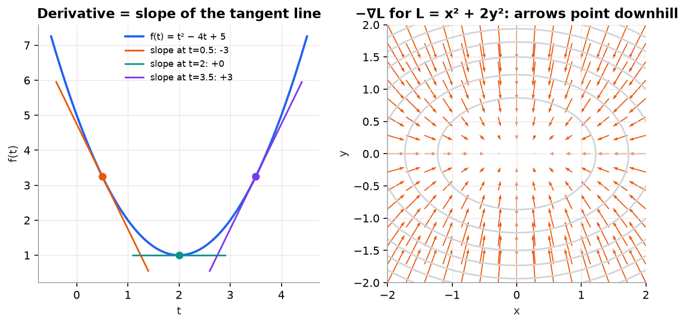
What to notice:
- The slope is zero exactly at the minimum, .
- On the right, arrows are longer where the surface is steeper and always cross contour lines at right angles. The direction is steeper (coefficient 2), so arrows lean vertically.
3. The math
Symbols
| Symbol | Meaning |
|---|---|
| or | derivative of with respect to |
| partial derivative of with respect to , others held fixed | |
| gradient: vector of all partial derivatives | |
| natural logarithm (base ) |
Rules you will use constantly
| Function | Derivative |
|---|---|
| (constant) | |
Chain rule. If and , then
Gradient. For , .
Worked example 1: a derivative
, so . At : and . Setting gives , the minimum, with .
Numerical check: . Always use this trick to test hand-derived gradients.
Worked example 2: partial derivatives and a gradient
. Treat as a constant to get ; treat as a constant to get . At : . The negative gradient points toward the origin, steeper in .
Worked example 3: the chain rule on squared error
For one example, with . Let .
With , , , : , so . A step with learning rate 0.1 gives , and the new prediction is 6, much closer to 7.
4. Implementation
You will compute derivatives numerically, use them to check an analytic gradient (the "gradient check" every framework author runs), and descend a loss surface. This is the core loop that gradient descent and backpropagation scale up.
Build it from scratch
A derivative is a slope, so measure it: nudge the input a tiny step each way and divide the change in output by the change in input. The central difference (x+h and x−h) is far more accurate than the one-sided version because the first-order errors cancel.
def derivative(f, x, h=1e-5):
    """Central difference: slope of the chord from x-h to x+h."""
    return (f(x + h) - f(x - h)) / (2 * h)
Predict: if you shrink h to 1e-15, does the estimate get better or worse? (Think about floating-point rounding when you subtract two nearly equal numbers.)
A gradient is one partial derivative per input. Nudge one coordinate at a time, holding the others fixed, exactly as in worked example 2.
def gradient(f, w, h=1e-5):
    """One central difference per coordinate: a vector of partial derivatives."""
    w = np.asarray(w, dtype=float)
    g = np.zeros_like(w)
    for i in range(w.size):
        e = np.zeros_like(w)
        e[i] = h
        g[i] = (f(w + e) - f(w - e)) / (2 * h)
    return g
Predict: a model with 1 million parameters. How many evaluations of the loss does this function need for one gradient? Why does that rule it out for training but not for testing?
Compare the numerical gradient to the analytic one you derived by hand. The relative error should be tiny (below about 1e-7); a value near 1e-2 means your formula has a bug.
def L(p):
    return p[0] ** 2 + 2 * p[1] ** 2

def grad_L(p):
    return np.array([2 * p[0], 4 * p[1]])            # analytic gradient
Gradient descent repeats one move: step against the gradient, scaled by the learning rate.
def descend(grad, w0, lr=0.1, steps=50):
    w = np.asarray(w0, dtype=float)
    for _ in range(steps):
        w = w - lr * grad(w)                         # step against the gradient
    return w
Predict: on , each step multiplies by . What happens to with lr = 0.6?
Answers
Tiny h makes it worse: f(x+h) and f(x-h) round to nearly the same float, and the difference is mostly rounding noise. Around 1e-5 is a good default for float64. One gradient costs 2 million loss evaluations (two per parameter), which is why training uses backpropagation (one forward and one backward pass) and numerical gradients only to test it. With lr = 0.6 the factor is 1 − 2.4 = −1.4: flips sign and grows 1.4× per step, so after 50 steps it is about 1.4⁵⁰ ≈ 2×10⁷. That is divergence; still converges because its factor is 1 − 1.2 = −0.2.
Use the library
Autograd frameworks compute exact gradients (up to float rounding), not approximations, by applying the chain rule through every operation you ran:
import torch

p = torch.tensor([1.0, 1.0], requires_grad=True)
(p[0] ** 2 + 2 * p[1] ** 2).backward()
print(p.grad)                     # tensor([2., 4.])
PyTorch records each operation in a graph during the forward pass, then walks it backward multiplying local derivatives. That is worked example 3 automated. torch.autograd.gradcheck runs the same numerical-versus-analytic comparison you just built.
Run it
From guide/:
uv run code/00-foundations/derivatives_scratch.pyf'(3): numerical 2.000000, analytic 2
∇L(1, 1): numerical [2. 4.], analytic [2. 4.], relative error 1.5e-12
chain rule dL/dw at w=1: -20.0, numerical -20.000000
one step, lr=0.1: w = 3.0, new prediction 6.0
gradient descent lr=0.1: from (1, 1) to [0. 0.]
gradient descent lr=0.6: from (1, 1) to [ 0. 20248916.2398]
all checks passThe chain-rule line reproduces worked example 3. Full script: code/00-foundations/derivatives_scratch.py. Figures: code/00-foundations/foundations.py.
5. Engineering
Gradient checking. Before trusting a hand-written gradient, compare it to finite differences on a few random inputs; relative error should be around or smaller. Frameworks use automatic differentiation, which is exact, so you mostly need this when writing custom operations.
Numerical issues. is and overflows. Libraries combine operations (log-softmax, BCE-with-logits) to stay stable; prefer them.
Where gradients vanish. The sigmoid's derivative is at most 0.25. Multiplying many such factors through the chain rule shrinks gradients toward zero in deep networks: the vanishing-gradient problem, covered in backpropagation.
Watch outFailure modes. Sign errors (stepping uphill), forgetting the inner derivative in the chain rule, and using a finite-difference step so small that floating-point rounding dominates.
Common mistakes
- Treating a partial derivative as if other variables also change.
- Dropping the factor 2 from a squared term (it only rescales the gradient, but it changes the effective learning rate).
- Confusing with ; ML formulas use natural logs unless stated.
6. Knowledge check
Quiz: Calculus for ML
For , what is ?
Practice exercise. For , compute and evaluate it at .
Solution
Chain rule: . At : .
Implementation challenge. Use numerical_grad to verify the analytic gradient of the linear-regression MSE () on random data.
Summary
- A derivative is a local slope; zero slope marks flat spots such as minima.
- Partial derivatives hold other inputs fixed; the gradient collects them and points uphill.
- The chain rule multiplies sensitivities along a chain of functions; backpropagation is this rule applied systematically.
- Check gradients with central finite differences.
Next: Probability and statistics
Related: Gradient descent · Backpropagation
Parts of this lesson are adapted from AI Engineering from Scratch by Rohit Ghumare (MIT license, notice): Calculus for Machine Learning.
Interview angle
Derive the derivative of the sigmoid and explain how it leads to vanishing gradients.
. Chain rule: . Split it as . The maximum is at , where and the derivative is ; at it is about . Backpropagation multiplies one such factor per sigmoid layer, so through 10 layers the gradient shrinks by at least , and far more if units saturate. Early layers stop learning. That is why hidden layers use ReLU-family activations (derivative 1 for positive inputs), along with careful initialization, normalization, and residual connections. Sigmoid is still fine at the output of a binary classifier when paired with cross-entropy, which cancels the term.
Why does the negative gradient point in the direction of steepest descent? When does following it work poorly?
For a small step , the first-order Taylor expansion is . Among all steps of fixed length , the change is most negative when , that is, when points exactly opposite the gradient. So is the locally steepest downhill direction, and its length is the slope. Two caveats interviewers look for. "Steepest" is measured in Euclidean distance in parameter space, so on badly scaled surfaces (like , or much worse ratios) the steepest direction does not point at the minimum and gradient descent zigzags; feature scaling and adaptive optimizers address this. And the guarantee is local: take too large a step and the linear approximation breaks, so the loss can go up.
You wrote a custom layer with a hand-derived backward pass, and the model trains poorly. How do you check your gradients?
Gradient checking with central differences. For each parameter , compute with , and compare with the analytic gradient using relative error . Around means correct; or worse means a bug. Practical details: run in float64, because in float32 rounding error dominates at small ; check a handful of random coordinates on a tiny input instead of every parameter; turn off dropout and other randomness so both evaluations see the same function; avoid kinks such as ReLU at exactly 0. Typical bugs it catches: a missing inner derivative in the chain rule, a sign error, a wrong sum over the batch dimension, a transposed matrix. PyTorch's torch.autograd.gradcheck automates this.
For L(w) = (wx − y)² with x = 2, y = 7, w = 1: what is the gradient, and what learning rate lands exactly on the optimum in one step?
The gradient is . The optimum is , so we need , giving . That is no coincidence: the second derivative is , and is the Newton step, which solves a quadratic in one move. The same curvature sets the stability limit: on a quadratic, gradient descent converges only if . At exactly it bounces between and forever; above it, it diverges. With many parameters, the largest curvature (the top Hessian eigenvalue) caps the learning rate while the smallest sets how slowly you crawl along flat directions. Their ratio, the condition number, explains why badly scaled problems train slowly.