Module 13: Deep-learning architectures 35 min6 min quick readDeep learning
Recurrent networks, LSTMs, and GRUs
Unroll an RNN through time by hand, explain why long dependencies are hard, see how LSTM and GRU gates help, and understand why transformers replaced them for language.
Before this: Backpropagation, The neural-network forward pass
Quick read: the intuition, interactive visualization, summary, and interview questions. The math, implementation, engineering, and knowledge-check sections are hidden.
Mental model. A recurrent network reads a sequence one step at a time and keeps a running summary, its hidden state. Each step combines the new input with the previous summary using the same weights.
You will learn to
- Write the RNN recurrence and unroll it for a short sequence by hand.
- Explain backpropagation through time and why gradients vanish or explode over long sequences.
- Describe the LSTM's cell state and gates, and the GRU's simplification.
- Compare RNNs with transformers on parallelism and long-range dependencies.
Why it matters. RNNs, LSTMs, and GRUs powered speech recognition and machine translation before transformers, and are still used for streaming and small-footprint time-series models. Their failure mode, vanishing gradients through time, motivated attention.
1. Intuition
To read "the cat that the dog chased ran away," you carry context forward: who is doing what. An RNN does the same with a vector . At each step it mixes the current word's embedding with the previous and squashes the result. The same weight matrices are used at every step (weight sharing across time, just like a CNN shares across space).
The problem: information from early steps has to survive many multiplications to influence a late step, and so does the gradient flowing back. If the effective multiplier per step is below 1, early information fades (vanishing gradients); above 1, it blows up.
LSTMs add a separate cell state, a conveyor belt that information can ride along with little change, controlled by gates that decide what to forget, what to write, and what to output. GRUs merge some gates for a simpler, similarly effective design.
2. Visualization
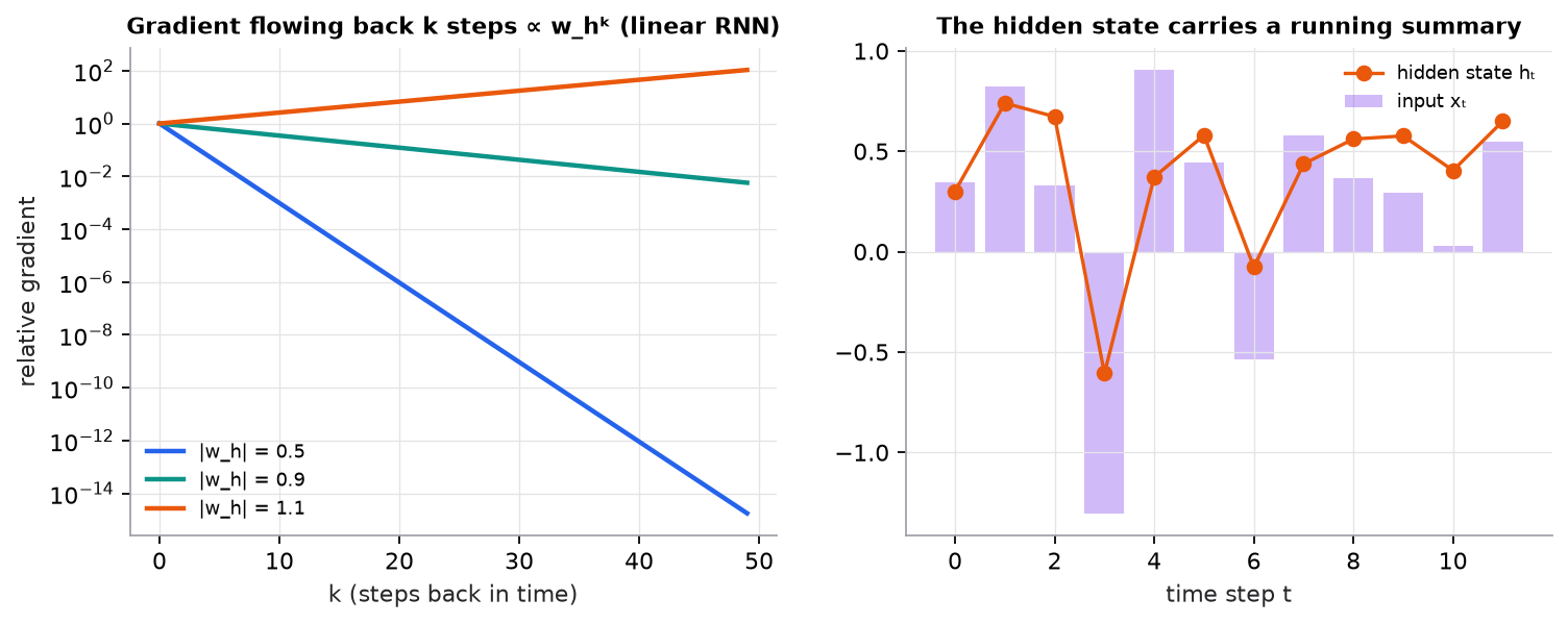
Synthetic. With a recurrent weight of 0.9, the gradient from 40 steps back is about of its original size; with 0.5 it is effectively zero after 15 steps.
3. The math
Symbols
| Symbol | Meaning | Shape |
|---|---|---|
| input at step | ||
| hidden state at step | ||
| input weights, recurrent weights, bias (shared across time) | , , | |
| LSTM cell state | ||
| forget, input, and output gates, each in | ||
| element-wise multiplication |
Vanilla RNN
Backpropagation through time
Unroll the network across all steps and backpropagate. The gradient from step to step includes a product of Jacobians, roughly . Its size behaves like the -th power of the recurrent weight's largest singular value times activation derivatives, which is why long dependencies vanish or explode.
LSTM
The key line is : when the forget gate is near 1, the cell state (and its gradient) passes through almost unchanged, like a residual connection through time.
Worked example: unrolling a scalar RNN
Scalar weights , , ; inputs ; .
| Pre-activation | ||
|---|---|---|
| 1 | ||
| 2 | ||
| 3 |
At there is no input, but the hidden state still remembers the first input (decaying from 0.46 to 0.35).
Gradient through time, linear simplification. Ignoring tanh, . After 30 steps, ; with it would be .
4. Implementation
The full script is code/13-deep-architectures/rnn_scratch.py (NumPy only). It builds a vanilla RNN, an LSTM cell, and a GRU cell, then measures the vanishing gradient directly.
Build it from scratch
Step 1: the vanilla RNN. The same tanh layer runs at every step, taking the current input and the previous hidden state. The loop is the point: step cannot start until step is done, which is why RNNs cannot be parallelized over time.
def rnn_forward(xs, Wx, Wh, b, h0):
    h, hs = h0, []
    for x in xs:                                   # sequential: step t needs step t-1
        h = np.tanh(Wx @ x + Wh @ h + b)
        hs.append(h)
    return np.stack(hs)                            # [T, d_h]
Predict: with the worked example's scalars (, , inputs ), what are ?
Step 2: the LSTM cell. One matrix multiply produces four blocks: forget gate f, input gate i, output gate o (all sigmoids, so between 0 and 1), and candidate g (tanh). The cell state c is updated by addition, not by passing through a squashing layer, and that is what lets gradients survive many steps.
def lstm_step(x, h, c, W, b):
    z = W @ np.concatenate([x, h]) + b             # all four blocks in one matmul: [4*d_h]
    f, i, o, g = np.split(z, 4)
    f, i, o, g = sigmoid(f), sigmoid(i), sigmoid(o), np.tanh(g)
    c = f * c + i * g                              # forget some old, write some new
    h = o * np.tanh(c)                             # expose a filtered view of c
    return h, c
Predict: if the forget gate is 1 and the input gate is 0 at every step, what happens to c? What is ?
Step 3: the GRU cell. Two gates and no separate cell state. The update gate z interpolates between keeping the old state and taking the new candidate; the reset gate r decides how much of the old state the candidate may look at.
def gru_step(x, h, W, U, b):
    zr = sigmoid(W[:2] @ x + U[:2] @ h + b[:2])    # update gate z, reset gate r (stacked)
    z, r = zr[0], zr[1]
    h_new = np.tanh(W[2] @ x + U[2] @ (r * h) + b[2])
    return (1 - z) * h + z * h_new                 # interpolate old and candidate
Predict: the LSTM has 4 weight blocks and the GRU 3. For the same sizes, what fraction of the LSTM's parameters does the GRU need?
Step 4: measure the vanishing gradient. By the chain rule, is a product of Jacobians, each . The script multiplies them out and takes the norm. Scaling an orthogonal controls how much each factor shrinks or stretches.
def grad_norm_to_start(Wh, T, rng, d_x=4):
    d_h = Wh.shape[0]
    Wx = rng.normal(scale=0.5, size=(d_h, d_x))
    h, J = np.zeros(d_h), np.eye(d_h)
    for _ in range(T):
        h = np.tanh(Wx @ rng.normal(size=d_x) + Wh @ h)
        J = np.diag(1 - h ** 2) @ Wh @ J           # dh_t/dh_0 = diag(tanh') Wh ... chain rule
    return np.linalg.norm(J, 2)
Predict: with exactly orthogonal (scale 1.0), every factor preserves length. Does the gradient still vanish? Why?
Use the library
nn.LSTM and nn.GRU run steps 2 and 3 over a whole batch and sequence, in cuDNN kernels. PyTorch orders the LSTM gates input, forget, candidate, output and keeps two bias vectors, so its count is per layer. Most implementations, PyTorch included, initialize the forget-gate bias to 0; setting it to 1 by hand (as the script does) is a common trick to start in "remember" mode.
import torch
from torch import nn

lstm = nn.LSTM(input_size=16, hidden_size=64, num_layers=2, batch_first=True)
out, (h_n, c_n) = lstm(torch.randn(8, 50, 16))
# out: [8, 50, 64]; h_n and c_n: [2, 8, 64]
Run it
uv run code/13-deep-architectures/rnn_scratch.pyKey lines of the output (weights and inputs are synthetic):
h_1..h_3: [0.4621 0.3537 0.8573]
linear gradient factors: 0.8^3 = 0.512  0.8^30 = 0.0012  1.1^30 = 17.4
LSTM h, c: (8,) (8,)  params: 416 (4 x d_h x (d_x + d_h + 1))
GRU h: (8,)  params: 312 (3 x d_h x (d_x + d_h + 1))
Wh = 0.5 x orthogonal: T=5 1.72e-02  T=20 1.76e-08  T=50 4.21e-21
Wh = 1.0 x orthogonal: T=5 4.15e-01  T=20 5.70e-03  T=50 2.56e-08
Wh = 1.5 x orthogonal: T=5 2.42e+00  T=20 1.17e+01  T=50 2.18e+00
LSTM cell path with forget gate 0.95: 0.95^50 = 0.077
The first two lines match the worked example. Even an orthogonal vanishes, because each tanh derivative is below 1. At scale 1.5 the gradient grows at first, then saturating tanh units cap it: the signal is unstable rather than cleanly exploding. The LSTM's additive path keeps 7.7% of the signal after 50 steps with a 0.95 forget gate, versus for the plain RNN. The script also includes a 1-D text CNN (a width-2 filter slid over word embeddings and max-pooled), the fast non-recurrent baseline for short-text classification. The figure script is code/13-deep-architectures/architectures.py.
5. Engineering
Where RNNs still fit. Streaming inputs where you must update a state per step with constant memory; tiny on-device models; some time-series forecasting. For tabular time series, gradient boosting on lagged features is often a stronger baseline.
Why transformers replaced them for language. RNNs must process tokens sequentially, so training can't be parallelized across time, and long-range information must survive many steps. Self-attention connects any two positions in one step and processes all positions in parallel during training. (Recent state-space models revisit recurrence with better long-range behavior.)
Sequence to sequence. For translation or summarization, an encoder RNN reads the whole input and hands its final hidden state to a decoder RNN, which generates the output one token at a time. That single fixed-size vector is a bottleneck: everything about a 50-word sentence must fit in, say, 512 numbers, and quality drops as inputs get longer. Attention was invented to fix exactly this: let the decoder look back at every encoder state, weighted by relevance, at each output step. Transformers then dropped the recurrence and kept the attention (see self-attention).
Training tips. Gradient clipping is standard; use LSTM or GRU cells rather than vanilla RNNs; truncated backpropagation through time limits memory for long sequences.
Watch outFailure modes. Exploding gradients (NaN losses) without clipping; forgetting information beyond a few dozen steps; slow training due to sequential computation; leakage in time-series evaluation through shuffled splits.
Common mistakes
- Using random splits for sequential data.
- Confusing
batch_firstlayouts ([B, T, F]versus[T, B, F]). - Assuming an LSTM's hidden state remembers arbitrarily long histories.
6. Knowledge check
Quiz: Recurrent networks, LSTMs, and GRUs
Scalar RNN with , , , , . What is the pre-activation ?
Practice exercise. Continue the worked example one more step with .
Solution
Pre-activation . .
Implementation challenge. Train a small LSTM and a vanilla RNN to remember the first token of a sequence and output it at the end, for sequence lengths 10, 50, and 100. Plot accuracy versus length for both.
Summary
- An RNN updates a hidden state with shared weights: .
- Backpropagation through time multiplies many factors, so gradients vanish or explode over long sequences.
- LSTMs and GRUs add gated paths (the cell state) that preserve information and gradients.
- Transformers replaced RNNs for language thanks to parallel training and direct long-range connections.
Next: Autoencoders, diffusion, and transfer learning
Related: Backpropagation · Self-attention · Model card: LSTM
Parts of this lesson are adapted from AI Engineering from Scratch by Rohit Ghumare (MIT license, notice): CNNs and RNNs for Text, Sequence-to-Sequence Models.
Interview angle
Why do vanilla RNNs struggle to learn long-range dependencies?
Because backpropagation through time multiplies the gradient by one Jacobian per step, and long products of the same factor vanish or explode. With , the gradient from step back to contains over steps. Its size behaves roughly like the -th power of 's largest singular value times the tanh derivatives, which are at most 1. In the scalar example with , is about ignoring tanh, but over 30 steps it is : the early input barely affects learning. With , and the gradients explode. Clipping handles explosion; vanishing needs an architectural fix, which is what LSTM gates and attention provide.
How does an LSTM's cell state fix the vanishing gradient problem?
It adds a path through time that is updated additively rather than by repeated matrix multiplication. The cell state updates as , so the direct derivative is just the forget gate , element-wise, with no weight matrix and no squashing derivative in the way. When the network learns for a unit, information and gradient pass through many steps almost unchanged, like a residual connection through time. The input gate decides what new content to write, and the output gate decides what to expose as . A GRU merges the gates into update and reset gates and drops the separate cell state, with fewer parameters and usually similar accuracy. Both extend usable memory to hundreds of steps, not arbitrarily far.
Transformers replaced RNNs for language. When would you still choose an RNN?
Transformers won on training: every position is computed in parallel, and any two tokens are one attention step apart instead of recurrent steps, so long-range dependencies are easier to learn. RNNs process steps sequentially, which underuses GPUs. But recurrence has an inference advantage: constant memory and constant compute per step, regardless of how long the stream has run. A transformer's KV cache and per-token attention cost grow with context length. So an RNN (LSTM or GRU) is still reasonable for streaming signals, on-device models with tight memory, low-latency time-series and sensor processing, and small datasets where a large transformer would overfit. State-space models and other linear-recurrent architectures revisit this trade-off: parallel training like a transformer, constant-size state at inference like an RNN. For text with any pretrained-model option available, I'd start with a transformer.
Your LSTM demand forecaster looks excellent in validation but performs poorly once deployed. What went wrong?
The most likely cause is temporal leakage in evaluation, not the model. Check the split first: a random or shuffled split lets the model train on days after the ones it is evaluated on, so it interpolates instead of forecasting. Use a time-based split or walk-forward validation that always trains on the past and tests on the future. Second, check feature construction: normalization statistics computed on the whole series, rolling features that include the current target, or inputs like actual weather that aren't known at prediction time all leak the future. Third, check for training-serving skew: production features computed by different code, arriving late, or missing. Finally, compare against a seasonal naive baseline (same period last week) on the honest split; if the LSTM barely beats it, a simpler model may be the better choice.