Module 13: Deep-learning architectures 40 min10 min quick readDeep learning
GANs, generator versus discriminator
Train a generator and a discriminator against each other, derive the optimal discriminator and the non-saturating loss, and diagnose mode collapse and vanishing gradients.
Before this: Autoencoders, diffusion, and transfer learning, Backpropagation, Loss functions
Quick read: the intuition, interactive visualization, summary, and interview questions. The math, implementation, engineering, and knowledge-check sections are hidden.
Mental model. A forger and a detective train together. The forger (generator) turns random noise into fake samples. The detective (discriminator) looks at real and fake samples and says how likely each one is to be real. Every time the detective learns a new tell, the forger gets a gradient that says "move your fakes this way". If they reach a stalemate where the detective can only guess, the fakes are distributed like the real data.
You will learn to
- Write the GAN minimax objective and the two alternating training steps, with shapes.
- Derive the optimal discriminator and explain the 0.5 equilibrium.
- Compute why the original generator loss saturates and the non-saturating loss doesn't.
- Implement a GAN with hand-written backprop and recognize mode collapse.
- Explain where adversarial training lives on in 2026: perceptual and adversarial losses in autoencoders and fast distilled diffusion samplers.
Why it matters. GANs introduced a way to learn a generator without writing down a likelihood: train a classifier to tell real from fake and use its gradient as the training signal. Diffusion and flow matching now produce the best open-domain images, but the adversarial idea stayed: Stable Diffusion's autoencoder is trained with an adversarial loss, and 1 to 4 step distilled samplers like SDXL-Turbo use one. GAN failure modes (mode collapse, a too-strong discriminator) are also classic interview material because they test whether you understand gradients, not just architectures.
1. Intuition
No likelihood, just a critic. An autoencoder trained with squared error averages over plausible outputs, which makes images blurry: the mean of many sharp faces is a blurry face. A GAN never measures pixel distance. Its generator only learns from whether the discriminator was fooled. A sample that looks plausible is rewarded, even if it matches no particular training image.
Two networks, alternating steps.
- Train for one step as an ordinary binary classifier: real samples labeled 1, generated samples labeled 0.
- Train for one step to make say "real" on fresh fakes. The gradient flows through (frozen for this step) into .
What the gradient means. 's output is a landscape over input space: high where it thinks real data lives. 's update moves each fake sample uphill on that landscape. As improves, must redraw the landscape. At equilibrium outputs 0.5 everywhere the data lives, so there is no uphill left.
Why it breaks. The game has no guarantee of converging. Two common failures:
- Vanishing gradient. If becomes too confident early, the original generator loss gives almost no gradient. The fix is the non-saturating loss (section 3).
- Mode collapse. finds one region currently accepts and puts all its samples there. 's gradient only acts where fakes are, so nothing pulls toward modes it never visits.
2. Visualization
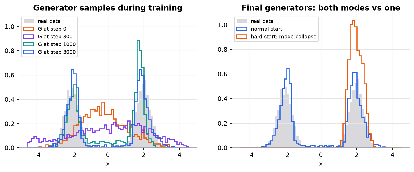
Synthetic data: a 50/50 mixture of Gaussians at and with standard deviation 0.4. Both networks are 2-hidden-layer MLPs with 32 units, trained with Adam in NumPy. In the hard-start run, 's output bias begins at 8 and is pre-trained for 300 steps: the fakes walk to the nearest real mode and stay there.
Try it (predict first, then run the script and check):
- In the normal run, and stay near 0.50 the whole time. Predict whether that means is useless, and what would do if stopped training.
- In the hard start, predict which mode the generator lands on and why it doesn't spread to the other one.
- Change
g_start=8.0tog_start=-8.0. Predict which mode wins now. - Call
train(1, non_saturating=False)from the normal start. Predict whether it still learns, then do the same with the hard start.
3. The math
Symbols
| Symbol | Meaning | Shape |
|---|---|---|
| a real sample | (here ) | |
| noise input to the generator, | (here 4) | |
| generator; outputs a fake sample | ||
| discriminator; probability that is real, of a logit | scalar in | |
| density of real data and of generator samples | functions of | |
| the game value | scalar |
The minimax game
The step maximizes , which is the same as minimizing binary cross-entropy with real = 1 and fake = 0:
The optimal discriminator
For a fixed , maximize at each point . Setting the derivative to 0, , gives
Substituting back in gives , where JSD is the Jensen-Shannon divergence. It is minimized, at , exactly when , and then everywhere.
Saturating versus non-saturating generator loss
The original generator loss is , to be minimized. The fix that Goodfellow et al. proposed in the same paper is to maximize instead:
With , the gradients with respect to the logit are
Worked example: a confident discriminator
Early in training easily rejects a fake: , logit .
- Saturating: .
- Non-saturating: .
Both point the same way, but the non-saturating gradient is times larger, exactly when most needs to move.
Worked example: one discriminator loss
on a real sample and on a fake.
The non-saturating generator loss on that fake is . At equilibrium, with everywhere, .
Worked example: optimal D at one point
At some , and : . is under-producing samples here, and the generator's gradient will push fakes toward this .
4. Implementation
The full script is code/13-deep-architectures/gan_scratch.py (NumPy only, about 4 seconds on a laptop CPU).
Build it from scratch
Step 1: the data and a small MLP. Real data is a two-mode mixture, shape [n, 1]. Both networks are the same MLP class: LeakyReLU hidden layers (no dead units for the generator's gradient to get stuck in) and a linear output. maps [n, 4] -> [n, 1]; maps [n, 1] -> [n, 1] logits.
def sample_real(rng, n):
    return (np.where(rng.random(n) < 0.5, -2.0, 2.0) + 0.4 * rng.standard_normal(n))[:, None]

    def forward(self, x):
        p = self.p
        a1 = x @ p["W1"] + p["b1"]
        h1 = np.where(a1 > 0, a1, 0.2 * a1)
        a2 = h1 @ p["W2"] + p["b2"]
        h2 = np.where(a2 > 0, a2, 0.2 * a2)
        self.cache = (x, a1, h1, a2, h2)
        return h2 @ p["W3"] + p["b3"]
Predict: what range of values can 's output take, and why doesn't 's forward end in a sigmoid?
Step 2: backprop that also returns the input gradient. The generator's update needs , the gradient with respect to 's input. So backward returns parameter gradients and d1 @ W1.T, the gradient flowing out of the first layer.
    def backward(self, d_out):
        x, a1, h1, a2, h2 = self.cache
        p = self.p
        g = {"W3": h2.T @ d_out, "b3": d_out.sum(0)}
        d2 = (d_out @ p["W3"].T) * np.where(a2 > 0, 1, 0.2)
        g["W2"], g["b2"] = h1.T @ d2, d2.sum(0)
        d1 = (d2 @ p["W2"].T) * np.where(a1 > 0, 1, 0.2)
        g["W1"], g["b1"] = x.T @ d1, d1.sum(0)
        return g, d1 @ p["W1"].T                  # parameter grads, input grad
Predict: the input gradient has which shape for a batch of 64 one-dimensional fakes?
Step 3: the discriminator step. Ordinary logistic regression on top of the MLP: stack real and fake, label 1 and 0. The gradient of binary cross-entropy with respect to the logit is sigmoid(logit) - label.
def d_step(D, real, fake, lr):
    x = np.vstack([real, fake])
    y = np.vstack([np.ones_like(real), np.zeros_like(fake)])
    p = sigmoid(D.forward(x))
    g, _ = D.backward((p - y) / len(x))
    D.adam(g, lr)
    return p[: len(real)].mean(), p[len(real):].mean()
Predict: in this step, does any gradient reach 's weights?
Step 4: the generator step. Fresh noise, a forward pass through then , the logit gradient from section 3, back through to its input, then back through . Only 's optimizer steps; 's weights are untouched.
def g_step(G, D, z, lr, non_saturating=True):
    fake = G.forward(z)
    p = sigmoid(D.forward(fake))
    # non-saturating: minimise -log D(G(z))   -> dL/dlogit = p - 1
    # saturating:     minimise log(1 - D(G(z))) -> dL/dlogit = -p
    d_logit = (p - 1) if non_saturating else -p
    _, d_fake = D.backward(d_logit / len(z))      # gradient flows through D to its input...
    g, _ = G.backward(d_fake)                    # ...then into G (D is NOT updated)
    G.adam(g, lr)
Predict: if you accidentally also called D.adam on these gradients, which way would move?
Step 5: the loop and a mode check. One step, then one step, 3,000 times. Adam uses (a common GAN default since DCGAN), since a lot of momentum makes the chase oscillate. The mode check counts samples within 1 of each mode.
        real = sample_real(rng, 64)
        fake = G.forward(rng.standard_normal((64, 4)))
        d_real, d_fake = d_step(D, real, fake, lr=1e-3)
        g_step(G, D, rng.standard_normal((64, 4)), lr=1e-3, non_saturating=non_saturating)

def coverage(xs):
    left = np.mean(np.abs(xs + 2) < 1)
    right = np.mean(np.abs(xs - 2) < 1)
    return left, right
Predict: a generator that outputs exactly every time. What does coverage return, and what would a single-number "sample quality" metric say about it?
Use the library
In PyTorch, autograd handles both backward passes. The two details to get right are fake.detach() in the step (so 's loss doesn't update ) and using the "real" label in the step (the non-saturating loss).
import torch, torch.nn as nn, torch.nn.functional as F

mlp = lambda i, o: nn.Sequential(nn.Linear(i, 32), nn.LeakyReLU(0.2), nn.Linear(32, 32), nn.LeakyReLU(0.2), nn.Linear(32, o))
G, D = mlp(4, 1), mlp(1, 1)
opt_g = torch.optim.Adam(G.parameters(), lr=1e-3, betas=(0.5, 0.999))
opt_d = torch.optim.Adam(D.parameters(), lr=1e-3, betas=(0.5, 0.999))
bce = F.binary_cross_entropy_with_logits                    # sigmoid + BCE, numerically stable

for real in loader:                                         # real: [B, 1]
    fake = G(torch.randn(len(real), 4))
    d_loss = bce(D(real), torch.ones_like(real)) + bce(D(fake.detach()), torch.zeros_like(real))
    opt_d.zero_grad(); d_loss.backward(); opt_d.step()
    g_loss = bce(D(fake), torch.ones_like(real))            # non-saturating: -log D(G(z))
    opt_g.zero_grad(); g_loss.backward(); opt_g.step()
For images, and become convolutional networks (DCGAN: strided convolutions, batch norm in , LeakyReLU in ), and stabilizers like spectral normalization in or a gradient penalty are standard.
Run it
uv run code/13-deep-architectures/gan_scratch.pyKey lines of output:
saturating     loss log(1 - D): d/dlogit = -D       = -0.010
non-saturating loss -log D:     d/dlogit = -(1 - D) = -0.990  (99x larger)

== Non-saturating GAN, 3000 steps ==
 step | D(real) | D(fake)
    1 |    0.52 |    0.51
 3000 |    0.50 |    0.50
mode coverage: 0.45 near -2, 0.51 near +2 (data: 0.50 / 0.50 minus tails)

== Hard start: G's samples begin near x = 8, D pre-trained 300 steps, 1500 steps ==
seed | D(fake) at start | near -2 | near +2
0 | 0.014 | 0.00 | 1.00hovers near 0.5 because keeps up with it on this easy 1-D problem; the useful signal is in the small, shifting slopes of , not its average. All three hard-start seeds collapse onto the mode.
5. Engineering
Where GANs stand in 2026. For open-domain text-to-image, video, and audio, diffusion and flow-matching models are the default: they train stably and cover the whole distribution. GANs remain strong in narrow domains (faces, a single product category, super-resolution) where their one-pass sampling is fast. The adversarial loss is everywhere:
- Autoencoders for latent diffusion. Stable Diffusion's autoencoder is trained with reconstruction, perceptual (LPIPS), and patch-based adversarial losses so decoded images are sharp (latent diffusion).
- Fast distilled samplers. SDXL-Turbo uses Adversarial Diffusion Distillation (an adversarial loss plus score distillation from a teacher) to sample in 1 to 4 steps; SD3-Turbo uses a latent variant. Not every fast sampler is adversarial: Latent Consistency Models use consistency distillation.
Stabilizers that matter. Non-saturating loss always. Adam with of 0 to 0.5. Spectral normalization on (bounds its slope). Wasserstein loss with gradient penalty (WGAN-GP) when overpowers . Two time-scale learning rates (TTUR: 's learning rate higher than 's). An exponential moving average of 's weights for sampling. Data augmentation applied to both real and fake inputs of when data is small.
Evaluation. Losses don't tell you sample quality: they're a game, not a target. Use FID (Fréchet distance between Inception features of real and generated sets; lower is better) on enough samples (it is biased at small sample counts, so compare at a fixed count such as 50,000), precision and recall for generative models (quality versus coverage separately), and look at sample grids. Mode collapse shows up as low recall and repeated samples.
Compute. Sampling is one forward pass of , so latency is low and fixed. Training is two networks, each step, and usually needs careful tuning per dataset.
Watch outA falling generator loss does not mean better samples. If 's accuracy goes to 100% and 's loss rises steadily, is getting no useful gradient; if 's outputs sit at 0.5 but samples look identical, you have mode collapse. Always look at samples and a coverage metric.
Common mistakes
- Forgetting
detach()on fakes in the step, so 's loss also trains in the wrong direction. - Reusing the -step fakes for the step after has updated, which gives stale gradients. Generate fresh fakes or recompute.
- Using the saturating loss .
- Letting batch norm see a batch of only real or only fake samples in and leak batch statistics; prefer spectral norm or layer norm in .
- Judging progress from loss curves instead of samples, FID, and coverage.
6. Knowledge check
Quiz: GANs, generator versus discriminator
What does the discriminator step of GAN training optimize?
Practice exercise. At a point , and . What is ? If a fake sits at this and outputs , what are the saturating and non-saturating gradients with respect to the logit?
Solution
. is over-producing here. Saturating: . Non-saturating: , four times larger. Both push the logit up (making the sample look more real), which in practice moves the fake toward regions where is higher, away from this over-crowded spot.
Implementation challenge. Extend the script to 2-D data: 8 Gaussians on a ring of radius 2. Count how many of the 8 modes have at least 5% of samples after 1,000, 3,000, and 6,000 steps. Then add minibatch standard deviation (append the batch's average standard deviation as an extra feature to 's input) and compare.
Hint
sample_real becomes angle for random , plus small Gaussian noise; takes [n, 2], outputs [n, 2]. For the minibatch feature, compute s = x.std(0).mean() and concatenate a column filled with s. Its gradient flows to every sample in the batch, so the backward pass needs a small extra term. If that's fiddly, stop the gradient through s first and see whether it still helps spot collapsed batches.
Summary
- A GAN trains to fool and to separate real from fake; learns from the gradient of , never from a likelihood.
- For fixed , ; at the global optimum and .
- Use the non-saturating loss ; its logit gradient is large exactly when is confident.
- Mode collapse happens because only shapes gradients where fakes already are; watch coverage and samples, not loss.
- In 2026 adversarial losses live on inside autoencoders and fast distilled diffusion samplers; diffusion and flow matching are the default generators.
Next: Latent diffusion and Stable Diffusion
Related: Autoencoders, diffusion, and transfer learning · Flow matching and rectified flows · Loss functions · Backpropagation
Go deeper, code-first (AI Engineering from Scratch): Conditional GANs & Pix2Pix
Parts of this lesson are adapted from AI Engineering from Scratch by Rohit Ghumare (MIT license, notice): GANs — Generator vs Discriminator.
Interview angle
Walk me through how a GAN trains. What is each network optimizing?
There are two networks. The generator maps noise z to a sample. The discriminator maps a sample to the probability that it's real. Training alternates. In the D step, D is an ordinary binary classifier: real samples labeled 1, generated samples labeled 0, minimizing binary cross-entropy, with the fakes detached so G isn't updated. In the G step, fresh fakes go through G and then D, and the loss is minus log D of G of z, which is minimized when D says real. The gradient flows back through D, whose weights are frozen for that step, into G. Formally it's a minimax game: for fixed G, the best D is p_data over p_data plus p_g, and plugging that in gives minus log 4 plus twice the Jensen-Shannon divergence, minimized when the generator's distribution equals the data's, where D outputs 0.5.
Why does the original generator loss saturate, and what does the non-saturating loss change?
The original game has G minimize log of one minus D of G of z. With D as a sigmoid of a logit a, the gradient with respect to a is minus D. Early in training, D easily rejects fakes, so D of G of z is near zero, and the gradient is near zero too: G learns almost nothing exactly when it's worst. The non-saturating loss instead minimizes minus log D of G of z. Its gradient with respect to the logit is minus one plus D, which is close to minus one when D is confident. At D equal to 0.01, the gradients are minus 0.01 versus minus 0.99, a 99 times difference, in the same direction. Both losses have the same fixed point, so you lose nothing in theory and gain a usable signal in practice. Goodfellow's original paper already recommended it.
Your GAN's samples all look nearly identical, but the losses look stable. Diagnose and fix.
That's mode collapse. Stable losses don't contradict it: G found a region D currently accepts and D's average output sits near 0.5. It happens because D only shapes gradients where fakes are; nothing pulls G toward modes it never visits, and G can hop between modes as D catches up. Confirm it with a coverage measure: precision and recall for generative models, FID at a fixed sample count, nearest-neighbor checks, or for toy data, counting samples per mode. Fixes, roughly in order: make D see batch-level statistics (minibatch standard deviation), stabilize D with spectral normalization or a gradient penalty, switch to a Wasserstein-style loss, lower G's learning rate or use two time-scale updates, average G's weights, and add augmentation if data is small. If coverage matters more than one-step speed, consider diffusion or flow matching instead.
GAN, diffusion, or flow matching for a product that must generate 512 by 512 product photos in under 50 ms on one GPU?
The constraint is latency: 50 milliseconds rules out a 30-step diffusion sampler at that resolution on typical hardware, since each step is a full network pass. Options. A GAN in a narrow domain (one product category, fixed backgrounds) gives a single forward pass and can be very sharp, but training is fiddly and coverage of rare variants is weaker. Or train a diffusion or flow-matching model, which is more stable and covers the distribution, then distill it to 1 to 4 steps with adversarial diffusion distillation or consistency distillation, so the adversarial loss is used as a distillation tool. I'd prototype the distilled latent model first, measure latency per step and FID plus human ratings against the GAN, and pick on measured quality and coverage at the 50 ms budget, not on reputation.