Module 13: Deep-learning architectures 40 min10 min quick readDeep learning
Flow matching and rectified flows
Train a generator by regressing a velocity field onto straight lines between noise and data, sample by integrating an ODE, see why one Euler step fails and how reflow straightens paths, and relate it all to diffusion.
Before this: Autoencoders, diffusion, and transfer learning, Calculus for ML, Gradient descent
Quick read: the intuition, interactive visualization, summary, and interview questions. The math, implementation, engineering, and knowledge-check sections are hidden.
Mental model. Pair every data point with a random noise point and draw a straight line between them. Train a network that, standing anywhere at any time, says which way and how fast to move: the average direction of all the lines passing through that spot. To generate, drop a particle at a noise point and follow the network's arrows back to data. The straighter the arrows' paths, the fewer steps you need.
You will learn to
- Write the flow-matching interpolant, its velocity target, and the training loss, with the time convention stated.
- Explain why the learned velocity is an average over crossing lines, and predict what a single Euler step produces.
- Implement flow-matching training and Euler sampling, and measure sample quality against step count.
- Explain rectified flow's reflow procedure and why it makes few-step sampling work.
- Convert between velocity, noise, and data predictions and relate flow matching to diffusion.
Why it matters. Flow matching is the training objective behind SD3, Flux, and many 2024 to 2026 image, video, and audio generators. It is simpler than diffusion (a plain regression on straight lines, no noise schedule algebra) and its straighter paths make few-step sampling and distillation easier. In interviews it shows up as "how does flow matching differ from diffusion?", which needs a precise answer.
1. Intuition
A straight-line recipe. Take a data point (say, 2.0) and a noise sample (say, ). The point slides along a straight line from data at to noise at . Its velocity is constant: . Training asks a network to predict that velocity from and alone.
Lines cross, so the network learns averages. Many (data, noise) pairs have lines passing through the same , heading in different directions. The best squared-error prediction is their average velocity. This average field is still exactly right in one sense: if you start from noise and follow it, the particles end up distributed like the data. But the paths it produces curve, because the average direction changes along the way.
Sampling is solving an ODE. Start at at and step backwards: . With straight paths, one big step would land exactly. With curved paths, big steps cut corners.
One step lands on the mean. At , is pure noise and says nothing about which data point it was paired with, so the averaged velocity points at the data mean. One Euler step from any noise sample lands near the mean of the data. For two modes at and , that's 0: a spike in the empty gap.
Reflow straightens. Run the trained model with many small steps to map each noise sample to a data sample. These pairs are no longer random: nearby noise goes to nearby data, so their lines rarely cross. Train a second model on those pairs, and its paths are nearly straight. Now one step works.
2. Visualization
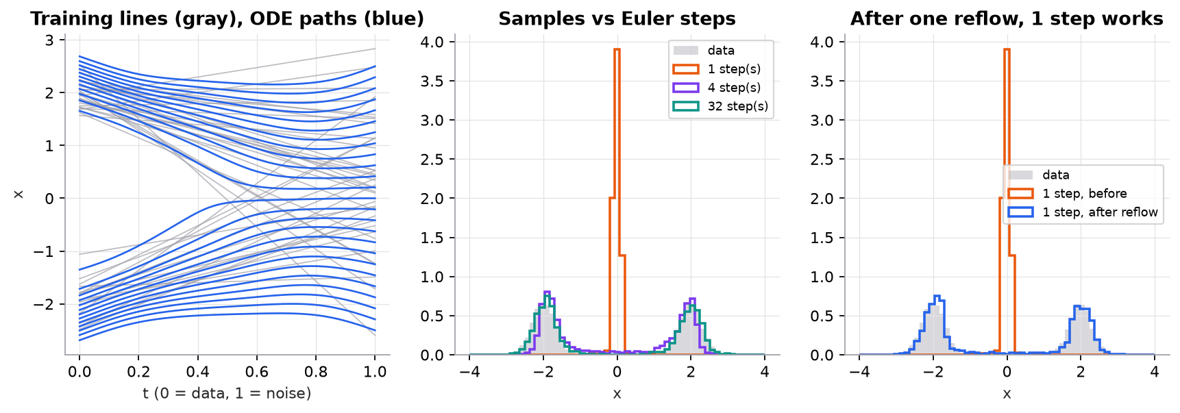
Synthetic data: a 50/50 mixture of Gaussians at and with standard deviation 0.3. The velocity network is a 2-hidden-layer tanh MLP with 64 units trained in NumPy. Learned paths (blue) can't cross, because an ODE has one velocity per point, so they curve where the straight training lines (gray) would cross.
Try it (predict first, then run the script and check):
- Predict the mean of 1-step samples from the first model, then check the "frac |x|>1" column.
- Predict how the 1-step error changes after reflow, and whether 4 steps after reflow is much better than 1.
- Shift the data so both modes sit at and . Predict where 1-step samples land.
- Train the first model with
steps=500instead of 3000. Predict whether 32-step sampling still looks good.
3. The math
Symbols
| Symbol | Meaning | Shape |
|---|---|---|
| data sample | ||
| noise sample | ||
| time; is data, is noise (the SD3 convention) | scalar | |
| point on the straight path | ||
| learned velocity field | ||
| ideal (marginal) velocity, the conditional average | ||
| Euler step size for steps | scalar |
Watch outPapers disagree on direction. Lipman et al. (2023) put noise at and data at ; rectified flow as used in SD3 puts data at . The math is identical with and a sign flip on . Check the convention before reusing code or a time-sampling scheme.
Interpolant and loss
This is conditional flow matching: the target uses the specific pair. Training is simulation-free: no ODE is solved during training.
What the network converges to
The minimizer of a squared loss is the conditional mean:
Following backward from produces exactly at (Lipman et al. 2023; Liu et al. 2022). The loss never reaches zero, because different pairs share the same ; the leftover is the variance of given .
At , , and is independent of , so . One Euler step of size 1 from gives : every sample lands on the data mean.
Sampling
Relation to diffusion
Diffusion with a Gaussian path writes . Rectified flow is the choice , , with . The three common prediction targets carry the same information:
So a velocity model is a diffusion model with a particular schedule and output parameterization. What changed in practice: straight interpolants, a simple constant target, and sampling as a deterministic ODE.
Rectified flow (reflow)
- Train with random pairs .
- For many , solve the ODE with (many small steps) to get .
- Train with the same loss on the coupled pairs .
The coupled pairs come from a non-crossing flow, so their straight lines rarely cross, and the new conditional average is close to each line's own velocity. Liu et al. show reflow never increases transport cost and makes paths straighter; one or two rounds usually suffice before distillation.
Worked example: one training pair
, , .
Going back to in one step along this pair's own line: , which recovers . The trained network won't output exactly here, because other pairs also pass through ; it outputs their average.
Worked example: one Euler step from noise
Data mean . For a noise sample : , so one step gives . The script's trained network gives against the theoretical , close enough that all 1-step samples land within 1 of zero.
4. Implementation
The full script is code/13-deep-architectures/flow_matching_scratch.py (NumPy only, about 3 seconds on a laptop CPU). The MLP class and Adam are the same pattern as in the GAN script.
Build it from scratch
Step 1: features for . The network sees position and time. Smooth functions of (sine and cosine) make it easier to represent velocity fields that change shape over time.
def features(x, t):
    # [n, 4]: position, time, and two Fourier features of time
    return np.stack([x, t, np.sin(np.pi * t), np.cos(np.pi * t)], axis=1)
Predict: if you dropped from the features entirely, what velocity would the network have to learn, and could it be right at both and ?
Step 2: the training step. Sample a time per example, build the point on the line, and regress onto the constant velocity. The gradient of mean squared error, 2 * (pred - target) / n, goes into the hand-written backward pass.
def fm_train_step(net, x0, x1):
    t = rng.random(len(x0))                  # t ~ Uniform(0, 1)
    xt = (1 - t) * x0 + t * x1               # a point on the straight line
    target = x1 - x0                         # its constant velocity
    pred = net(xt, t)
    loss = np.mean((pred - target) ** 2)
    net.adam(net.backward(2 * (pred - target) / len(x0)))
    return loss
Predict: the final loss is 2.301, not 0. Is the model underfitting? (Hint: section 3, "what the network converges to".)
Step 3: random pairing. For the first model, data and noise are drawn independently: train(net, lambda n: (sample_data(n), rng.standard_normal(n))). The pairing function is the only thing reflow will change.
def train(net, pairs_fn, steps=3000, batch=256):
    for _ in range(steps):
        x0, x1 = pairs_fn(batch)
        loss = fm_train_step(net, x0, x1)
    return loss
Predict: with independent pairs, how often do two training lines cross?
Step 4: Euler sampling. Start at noise, step from down to . Each step evaluates the network once, so n_steps is the cost.
def sample(net, x1, n_steps, keep_path=False):
    x, dt = x1.copy(), 1.0 / n_steps
    path = [x.copy()]
    for i in range(n_steps):
        t = np.full_like(x, 1.0 - i * dt)    # integrate from t = 1 (noise) to t = 0 (data)
        x = x - dt * net(x, t)               # Euler step
        path.append(x.copy())
    return (x, np.array(path)) if keep_path else x
Predict: with n_steps=2, at which two times is the network evaluated?
Step 5: reflow. Map 20,000 noise samples through the first model with 64 steps, then train a fresh model on those coupled pairs. Indexing both arrays with the same idx keeps each pair together.
    z_pairs = rng.standard_normal(20000)
    x_pairs = sample(net, z_pairs, 64)                    # deterministic ODE couples z -> x
    net2 = MLP()

    def coupled(n):
        idx = rng.integers(0, len(z_pairs), n)
        return x_pairs[idx], z_pairs[idx]

    train(net2, coupled)
Predict: if you shuffled x_pairs before training net2, what would reflow do?
Use the library
There's no one-line flow-matching layer; the training loop is short enough to write in PyTorch directly. Production models use the same loss with a transformer for , latents instead of pixels, a conditioning input, and non-uniform time sampling.
import torch

def fm_loss(model, x0, cond):                     # x0: [B, C, H, W] latents
    x1 = torch.randn_like(x0)
    t = torch.sigmoid(torch.randn(x0.shape[0], device=x0.device))   # logit-normal t, as in SD3
    tt = t.view(-1, 1, 1, 1)
    xt = (1 - tt) * x0 + tt * x1
    return torch.nn.functional.mse_loss(model(xt, t, cond), x1 - x0)
For sampling, diffusers ships FlowMatchEulerDiscreteScheduler, which SD3 and Flux pipelines use; num_inference_steps is . The torchcfm package provides conditional flow matching variants, including minibatch optimal-transport pairing, another way to get straighter paths without a full reflow.
Run it
uv run code/13-deep-architectures/flow_matching_scratch.pyKey lines of output:
x0 = 2.0, x1 = -0.5, t = 0.25:  x_t = 1.375, target velocity = -2.500
one Euler step back to t = 0: x_t - t * v = 2.000 (recovers x0)
final training loss: 2.301 (cannot reach 0: one x_t has many possible x1 - x0)
v(x=0, t=1) = -0.011   v(x=1, t=1) = +1.114   (theory: v(x, 1) = x - E[x0] = x)
steps | W1 to data | frac |x|>1
    1 |      1.920 |       0.00
    2 |      0.687 |       0.72
    4 |      0.276 |       0.92
    8 |      0.147 |       0.97
   32 |      0.068 |       0.99

steps | W1 before | W1 after reflow
    1 |     1.920 |           0.081
    4 |     0.276 |           0.078
W1 is the 1-D Wasserstein distance to fresh data samples (mean gap between sorted samples; lower is better). Before reflow, error falls steadily with steps. After one reflow, 1 step is already as good as 32 steps of the original model.
5. Engineering
Why it took over. Training is a stable regression with a simple target. Straighter paths make deterministic ODE samplers efficient (20 to 30 steps instead of hundreds) and give distillation a better starting point. SD3 reported that rectified flow with logit-normal time sampling (more training on middle times, where prediction is hardest) beat other diffusion formulations at scale in their experiments.
Time sampling. Uniform wastes effort near and , where the target is easy to predict. Logit-normal sampling, with , concentrates on the middle. At high resolution, models also shift the schedule toward noisier times, because more pixels mean more redundant signal survives a given noise level.
Getting to few steps. Options, from cheapest to most involved: a better ODE solver (Heun, midpoint) at the same number of evaluations; reflow (costs a full generation pass over a large set of noise samples to build pairs); and distillation into a 1 to 4 step student (consistency-style or adversarial). Fast open models such as Flux.1-schnell are flow-matching models distilled to a few steps.
Guidance. Classifier-free guidance works on velocities just as on noise: (see latent diffusion).
Beyond images. The same recipe trains audio, video, molecule, and robot-action generators: anything where you can draw samples and need a generator that maps noise to data.
Common mistakes
- Mixing time conventions (data at versus ) between training and sampling, which flips the velocity sign.
- Expecting a model trained with random pairs to sample well in 1 step: that lands on the data mean.
- Reading the training loss as sample quality. Its floor is the irreducible variance of crossing lines; compare sample metrics across step counts.
- Shuffling or mismatching pairs when building a reflow dataset, which throws away the coupling.
- Evaluating at only one step count; report quality versus number of function evaluations.
6. Knowledge check
Quiz: Flow matching and rectified flows
With ( data, noise), what does a conditional flow-matching network regress onto?
Practice exercise. A velocity model is trained with . At , , and the model predicts . What are its implied predictions and ? Then take one Euler step of size .
Solution
. . Check: . Euler step to : .
Implementation challenge. Replace Euler with Heun's method (predict with Euler, evaluate the velocity at the predicted point, average the two velocities) in sample. Compare W1 at an equal number of network evaluations: Euler with 8 steps versus Heun with 4 steps (also 8 evaluations).
Hint
One Heun step from to : ; ; ; . Skip the second evaluation on the last step if is outside the range you trained well.
Summary
- Flow matching regresses onto along straight lines ; training needs no ODE solves.
- The network learns the average velocity of all lines through a point; following it from noise reproduces the data distribution.
- With random pairs, paths curve and one Euler step lands on the data mean; quality improves with more steps.
- Reflow retrains on the model's own (noise, sample) pairs, straightening paths so 1 to 2 steps work; distillation goes further.
- Velocity, noise, and data predictions are interchangeable; rectified flow is diffusion with a straight-line schedule. SD3 and Flux use it.
Next: Object detection and YOLO
Related: Latent diffusion and Stable Diffusion · GANs · Autoencoders, diffusion, and transfer learning · Model card: diffusion model
Go deeper, code-first (AI Engineering from Scratch): Diffusion Transformers & Rectified Flow
Parts of this lesson are adapted from AI Engineering from Scratch by Rohit Ghumare (MIT license, notice): Flow Matching & Rectified Flows.
Interview angle
What is flow matching, and how is it trained?
Flow matching learns a velocity field that carries noise to data. Pick a data sample x0 and a noise sample x1, and a time t between 0 and 1. The point x_t equals one minus t times x0 plus t times x1 lies on a straight line, and its velocity is the constant x1 minus x0. Train a network v of x_t and t to predict that velocity with mean squared error. No ODE is solved during training, so it's as simple as supervised regression. Because many pairs pass through the same point, the network learns their average velocity, which is still the right field: integrating it backwards from Gaussian noise yields the data distribution. To sample, start at noise and take Euler or higher-order steps from t equals 1 to 0. SD3 and Flux train this way in a latent space with a transformer predicting the velocity.
How does flow matching relate to diffusion? Is it a different kind of model?
It's closely related. A Gaussian diffusion path is x_t equals alpha_t times x0 plus sigma_t times epsilon. Rectified flow is the special case alpha equals one minus t and sigma equals t, with epsilon as the noise endpoint. A network that predicts velocity, noise, or clean data carries the same information: x0-hat equals x_t minus t v, and epsilon-hat equals x_t plus one minus t times v. So a flow-matching model is a diffusion model with a straight-line schedule and a velocity parameterization, sampled with a deterministic ODE. What changed in practice: the target is simple and well-scaled across time, paths are straighter so samplers need fewer steps, and the framework allows non-Gaussian endpoints and custom couplings. The SD3 paper found rectified flow with logit-normal time sampling compared favorably to other formulations at scale.
Your flow-matching model samples well with 30 steps but gives blurry, averaged outputs with 1 to 2 steps. Why, and what are your options?
That's expected for a model trained with independent noise-data pairs. Lines from different pairs cross, so the learned velocity at a point is an average, and the true paths curve. A single big Euler step follows the initial direction, and at t equals 1 that direction points at the conditional mean of the data, which for images is a blurry average. In the course toy, 1-step samples all land near zero between two modes. Options. Use a better solver, such as Heun, at the same number of evaluations. Do one or two rounds of reflow: generate (noise, sample) pairs with the current model and retrain on them, which straightens paths; in the toy one reflow cut 1-step error from 1.92 to 0.08. Use minibatch optimal-transport pairing during training. Or distill into a few-step student with consistency or adversarial distillation.
Compute a velocity model's implied clean-data prediction at t equal to 0.6, x_t equal to 0.8, v equal to minus 1.5, and take an Euler step of 0.2.
With the convention x_t equals one minus t times x0 plus t times x1, the velocity is x1 minus x0, so x0-hat equals x_t minus t times v. That's 0.8 minus 0.6 times minus 1.5, which is 0.8 plus 0.9, or 1.7. The implied noise is x_t plus one minus t times v: 0.8 plus 0.4 times minus 1.5, which is 0.8 minus 0.6, or 0.2. Check it: 0.4 times 1.7 plus 0.6 times 0.2 is 0.68 plus 0.12, which is 0.8. One Euler step toward data with step 0.2: x becomes 0.8 minus 0.2 times minus 1.5, which is 1.1, now at t equals 0.4. If the path were perfectly straight, two more such steps would land exactly on 1.7; curvature is what makes that estimate drift.