Module 13: Deep-learning architectures 40 min10 min quick readDeep learning
Latent diffusion and Stable Diffusion
Explain why Stable Diffusion runs diffusion in an autoencoder's latent space, how text enters through cross-attention, and how classifier-free guidance trades diversity for prompt adherence; build a toy latent diffusion model with guidance.
Before this: Autoencoders, diffusion, and transfer learning, Self-attention, PCA, t-SNE, and UMAP
Quick read: the intuition, interactive visualization, summary, and interview questions. The math, implementation, engineering, and knowledge-check sections are hidden.
Mental model. Don't paint every pixel from scratch. First train a compressor that turns an image into a small "sketch" (a latent) and back. Then teach a diffusion model to draw sketches. At generation time, the diffusion model denoises a random sketch into a good one, guided by the text prompt, and the decompressor paints the pixels. All the expensive iterative work happens on the small sketch.
You will learn to
- Describe the two stages of latent diffusion (a frozen autoencoder, then diffusion on its latents) and compute the compression for common models.
- Explain why latents are rescaled to unit variance and what goes wrong if you forget.
- Explain how text conditions the denoiser through cross-attention, and what changed from U-Nets to diffusion transformers.
- Derive and apply classifier-free guidance, including how the guidance scale is defined in code.
- Build a toy latent diffusion model with label dropout and a guidance sweep.
Why it matters. Stable Diffusion, SDXL, SD3, and Flux all follow this recipe, and most open image and video generators build on it. Interviewers ask about it because it combines three ideas you already know (autoencoders, diffusion, attention) into one system with clear engineering trade-offs: compression versus detail, guidance versus diversity, and steps versus latency.
1. Intuition
Pixels are wasteful. A 512 by 512 RGB image has 786,432 numbers, but most of them encode fine texture that a good compressor can store compactly. Diffusion runs its network dozens of times per image, so every number it has to process costs that many times over.
Stage 1: learn a compressor once. An autoencoder with encoder and decoder maps the image to a latent 8 times smaller in each spatial direction, with a few channels: 512 by 512 by 3 becomes 64 by 64 by 4. It is trained for reconstruction, with a perceptual loss and an adversarial loss so decoded images are sharp (see GANs), and a small KL penalty that keeps the latent space smooth. Then it is frozen.
Stage 2: diffusion on latents. Treat as the data. Training is exactly the noise-prediction recipe from the diffusion lesson: add noise to , ask the network to predict the noise. At generation time: sample pure noise in latent space, denoise it step by step, then decode once with .
Text gets in through attention. A frozen text encoder (CLIP, later also T5) turns the prompt into a sequence of token vectors. Inside the denoiser, image features ask questions (queries) and the text tokens answer (keys and values): cross-attention. That is how "a red bicycle" changes which noise gets removed.
Guidance turns up the prompt. During training the prompt is sometimes dropped, so one network learns both "denoise given this prompt" and "denoise with no prompt". At sampling time you compute both and push further in the direction of their difference. More push means images that match the prompt more strongly, with less variety, and eventually oversaturated artifacts.
2. Visualization
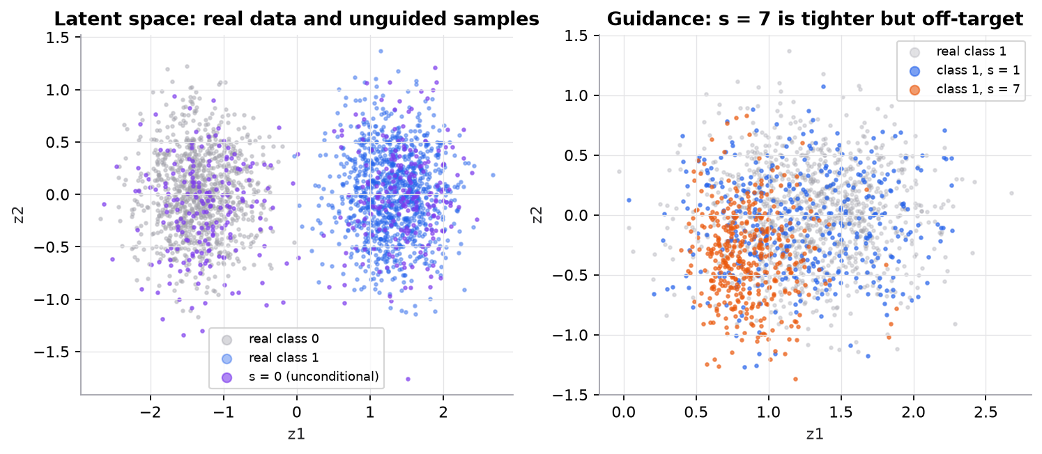
Synthetic data: 16-dimensional "images" that lie near a 2-D plane, in two classes. Stage 1 is PCA (a linear autoencoder) with a scaling factor; stage 2 is a small class-conditional noise-prediction MLP with 10% label dropout, trained only on the 2-D latents. Scale 0 ignores the label; scale 1 matches the class; scale 7 is tighter but off target.
Try it (predict first, then run the script and check):
- Scale 0 uses only the unconditional prediction. Predict the mean latent of scale-0 samples and check it against the table.
- Predict how the spread (standard deviation) of class-1 samples changes from scale 1 to 7, then check.
- Set
p_uncond=0.0intrain_step. Predict what the "unconditional" prediction becomes, and what guidance does then. - Remove
* SCALEfromencode(and/ SCALEfromdecode). Predict what happens to samples, given that steps end in noise of standard deviation about 1.
3. The math
Symbols
| Symbol | Meaning | Shape (SD 1.5) |
|---|---|---|
| image | ||
| frozen encoder and decoder | ||
| scaled latent; is the scaling factor | ||
| noised latent at step | ||
| noise schedule; | scalars | |
| conditioning: text token embeddings, or for none | for SD 1.5 | |
| network's noise prediction | ||
| guidance scale (as used in code) | scalar |
Training
Same loss as pixel diffusion, on latents:
with replaced by (empty prompt) about 10% of the time.
Cross-attention
Image features (one row per latent position) attend to text tokens :
For a 64 by 64 latent at full resolution, has 4,096 rows and have 77 rows, so the attention matrix is 4,096 by 77. Each latent position gets a weighted mix of prompt tokens.
Classifier-free guidance
is unconditional, is the plain conditional model, and extrapolates past it. The original paper writes it as , which is the same thing with . Libraries like diffusers use the first form (guidance_scale, default 7.5 for SD 1.5), so check which convention a paper uses before copying a number.
Worked example: compression
| Model | Image values | Latent values | Ratio |
|---|---|---|---|
| SD 1.5 | |||
| SDXL | |||
| SD3, Flux |
Spatial positions drop times (262,144 pixels to 4,096 latent positions for SD 1.5), which is what drives the cost of convolutions and self-attention. The move from 4 to 16 channels in SD3 and Flux keeps more detail at the same spatial size.
Worked example: scaling factor
SD 1.5's autoencoder outputs latents with standard deviation of roughly 5.5. The diffusion schedule assumes data of about unit variance, because at the last step with standard deviation 1. So latents are multiplied by : . SDXL's autoencoder uses . In the toy script, the PCA latents have standard deviation 5.170, so , and the scaled latents have standard deviation 1.000.
Worked example: one guidance step
For one latent value, and , with :
The guided prediction lies beyond both raw predictions, which is why large overshoots: in the script, pushes class-1 samples to a mean 0.56 away from the real class centre, versus 0.10 at .
4. Implementation
The full script is code/13-deep-architectures/latent_diffusion_scratch.py (NumPy only, about 4 seconds on a laptop CPU).
Build it from scratch
Step 1: data that lives near a low-dimensional surface. Real images occupy a tiny part of pixel space, which is why compression works. We imitate that: 2-D class clusters, embedded in 16 dimensions by a fixed random basis, plus a little noise.
BASIS = np.linalg.qr(rng.standard_normal((D_PIX, D_LAT)))[0].T * 6.0   # [2, 16]
CENTERS = np.array([[-1.0, 0.5], [1.0, -0.5]])                          # class centres in the plane

def sample_data(n):
    c = rng.integers(0, 2, n)
    plane = CENTERS[c] + 0.35 * rng.standard_normal((n, D_LAT))
    return plane @ BASIS + 0.05 * rng.standard_normal((n, D_PIX)), c    # [n, 16], [n]
Predict: how many principal components will capture almost all the variance of this data?
Step 2: stage 1, a frozen linear autoencoder with a scaling factor. PCA is the optimal linear autoencoder (PCA lesson). The top 2 directions form the encoder, their transpose the decoder. SCALE brings latents to unit standard deviation, playing the role of SD's 0.18215.
X_fit, _ = sample_data(5000)
MU = X_fit.mean(0)
ENC = np.linalg.svd(X_fit - MU, full_matrices=False)[2][:D_LAT].T     # [16, 2] top principal directions
Z_raw = (X_fit - MU) @ ENC
SCALE = 1.0 / Z_raw.std()                                              # like SD's VAE scaling factor

def encode(x):
    return (x - MU) @ ENC * SCALE          # [n, 16] -> [n, 2], roughly unit variance

def decode(z):
    return (z / SCALE) @ ENC.T + MU        # [n, 2] -> [n, 16]
Predict: the script prints reconstruction MSE 0.0022 against a per-dimension data variance of 3.46. Where does the remaining error come from?
Step 3: stage 2 training, on latents, with label dropout. The data is encoded first, so the denoiser never sees 16-D vectors. Ten percent of labels are swapped for the null class id, so the same network learns the unconditional prediction.
def train_step(net, batch=256, p_uncond=0.1):
    x0, c = sample_data(batch)
    z0 = encode(x0)                                      # diffusion never sees the 16-D data
    t = rng.integers(0, T, batch)
    eps = rng.standard_normal(z0.shape)
    zt = np.sqrt(abar[t])[:, None] * z0 + np.sqrt(1 - abar[t])[:, None] * eps
    c = np.where(rng.random(batch) < p_uncond, NULL, c)   # label dropout: learn eps_uncond too
    pred = net.forward(features(zt, t, c))
    net.adam(net.backward(2 * (pred - eps) / pred.size))
    return np.mean((pred - eps) ** 2)
Predict: the loss plateaus near 0.2 rather than 0. Is the network failing? (Hint: at small , how much can anyone tell about from ?)
Step 4: sampling with guidance, then decode. Two network calls per step (conditional and null), combined with the guidance formula, then the standard DDPM update. The decoder runs once at the end, outside this loop.
def sample(net, c, s, n):
    z = rng.standard_normal((n, D_LAT))
    cc, cu = np.full(n, c), np.full(n, NULL)
    for t in range(T - 1, -1, -1):
        tt = np.full(n, t)
        e_c = net.forward(features(z, tt, cc))
        e_u = net.forward(features(z, tt, cu))
        e = e_u + s * (e_c - e_u)                        # CFG
        z = (z - betas[t] / np.sqrt(1 - abar[t]) * e) / np.sqrt(alphas[t])
        if t > 0:
            z += np.sqrt(betas[t]) * rng.standard_normal(z.shape)
    return z
Predict: guidance doubles the number of network calls per step. How do real pipelines avoid doubling latency? (Hint: the batch dimension.)
Use the library
diffusers wraps the text encoders, denoiser, scheduler, and autoencoder in one pipeline. guidance_scale is in the formula above; a negative prompt replaces the empty prompt in the unconditional branch.
import torch
from diffusers import AutoPipelineForText2Image

pipe = AutoPipelineForText2Image.from_pretrained(
    "stabilityai/stable-diffusion-xl-base-1.0", torch_dtype=torch.float16).to("cuda")
image = pipe("a red bicycle leaning on a brick wall, golden hour",
             negative_prompt="blurry, low quality",
             num_inference_steps=30, guidance_scale=7.0).images[0]

# Stage 1 by hand: encode an image tensor in [-1, 1], shape [1, 3, 1024, 1024]
latents = pipe.vae.encode(x).latent_dist.sample() * pipe.vae.config.scaling_factor   # [1, 4, 128, 128]
What the library adds over the toy: a convolutional autoencoder, a U-Net or transformer denoiser with cross-attention, better samplers that need 20 to 50 steps, batched conditional and unconditional passes, and memory options such as enable_model_cpu_offload().
Architecture lineage (open models).
| Model | Year | Denoiser | Latent at native size | Text encoders | Training objective |
|---|---|---|---|---|---|
| SD 1.5 | 2022 | U-Net, about 860M | (512 px) | CLIP ViT-L/14 | noise prediction |
| SD 2.x | 2022 | U-Net | (768 px) | OpenCLIP ViT-H | v-prediction |
| SDXL | 2023 | larger U-Net | (1024 px) | CLIP ViT-L + OpenCLIP ViT-bigG | noise prediction |
| SD3 | 2024 | MMDiT (transformer) | CLIP-L, OpenCLIP bigG, T5-XXL | rectified flow | |
| Flux.1 | 2024 | rectified-flow transformer, 12B | 16 channels | CLIP-L, T5-XXL | rectified flow |
The trend: transformers over latent patches replace the U-Net, larger text encoders (T5) improve prompt following and text rendering, more latent channels keep more detail, and the training objective moves to flow matching.
Run it
uv run code/13-deep-architectures/latent_diffusion_scratch.pyKey lines of output:
     SD 1.5, 512px:   786,432 pixel values ->  16,384 latent values = 48x fewer
latent std before scaling: 5.170, scale factor: 0.1934, after: 1.000
eps_uncond = 0.2, eps_cond = 0.5, s = 3.0: eps = 0.2 + 3.0 * (0.5 - 0.2) = 1.10

real class-1 latents: mean [1.3  0.01], spread 0.40
scale s |     mean latent | spread | dist to centre
    0.0 |   [ 0.12 -0.07] |   0.93 |           1.18
    1.0 |   [ 1.24 -0.07] |   0.44 |           0.10
    3.0 |   [ 1.14 -0.18] |   0.38 |           0.25
    7.0 |   [ 0.87 -0.35] |   0.31 |           0.56
Scale 0 averages both classes (mean near 0, wide spread). Scale 1 matches the real class. Larger scales shrink the spread and drift off target: that's the diversity-for-adherence trade, taken too far. Real image models usually need above 1 because their conditional prediction alone follows prompts weakly; this toy's labels are easy.
5. Engineering
Choosing the guidance scale. Typical defaults are around 5 to 8 for SD-family models. Too low: images ignore parts of the prompt. Too high: oversaturated colors, harsh contrast, and repeated compositions. Distilled few-step models (Turbo, Schnell, LCM) are usually run with guidance off or very low, because guidance was baked in during distillation.
Latency and memory. Cost is roughly (number of steps) times (one denoiser pass, doubled by guidance unless batched) plus one decoder pass. Levers: fewer steps with a better sampler, distillation to 1 to 4 steps, fp16 or bf16 weights, quantization, attention kernels such as FlashAttention, and offloading text encoders (T5-XXL is large) to CPU once the prompt is encoded.
Fine-tuning. LoRA adapters on the denoiser's attention layers are the standard way to teach a style or subject (fine-tuning in practice). ControlNet and adapters add spatial conditions (edges, depth, pose). All of these are tied to one base model's latent space and architecture.
Safety and provenance. Open models need filters on prompts and outputs, and many products add invisible watermarks or C2PA metadata. Training data licensing is an active legal area; check a model's license before commercial use.
Watch outLatent spaces are not interchangeable. SD 1.5, SDXL, SD3, and Flux each have their own autoencoder and scaling factor. A LoRA, ControlNet, or set of precomputed latents for one will not work with another. Decoding latents with the wrong autoencoder or forgetting to divide by the scaling factor produces garbage or washed-out images.
Common mistakes
- Forgetting the scaling factor when encoding training data or decoding samples.
- Confusing the two CFG conventions and setting when you meant "no guidance" in the convention.
- Training without condition dropout, then trying to use classifier-free guidance.
- Mixing components across model families (VAE, text encoder, LoRA).
- Measuring quality on a handful of cherry-picked images; use a fixed prompt set, FID or CLIP-based scores, and human ratings.
6. Knowledge check
Quiz: Latent diffusion and Stable Diffusion
SD 1.5 encodes a image into a latent. How many times fewer values does the diffusion model process?
Practice exercise. A video model encodes 16 frames of into a latent of shape (channels, frames, height, width). How many times fewer values does diffusion process, and what is the spatial downsampling factor per side?
Solution
Pixels: . Latent: . Ratio . Spatial downsampling per side, and no compression in time. Many video autoencoders also compress time (for example 4 times), which would make the ratio 192.
Implementation challenge. Replace the PCA autoencoder with a small nonlinear autoencoder (one tanh hidden layer each way) trained with reconstruction loss, on data that lies on a curved 2-D surface instead of a plane (for example, add 0.3 * plane[:, :1]**2 along a third basis direction). Compare reconstruction error and guided samples against PCA.
Hint
PCA can only find flat subspaces, so a curved surface needs 3 linear components where a nonlinear autoencoder needs 2. Remember to recompute the scaling factor from the new encoder's latents, and train stage 2 only after freezing stage 1.
Summary
- Latent diffusion trains an autoencoder once, freezes it, and runs diffusion on its latents: 48 times fewer values and 64 times fewer spatial positions for SD 1.5 at 512 px.
- Latents are scaled to unit variance (0.18215 for SD 1.5) so the noise schedule fits the data.
- Text enters the denoiser through cross-attention: image positions are queries, text tokens are keys and values.
- Classifier-free guidance, , trades diversity for prompt adherence; too large overshoots.
- SD3 and Flux keep the latent recipe but use transformers, 16-channel latents, T5 text encoders, and rectified flow.
Next: Flow matching and rectified flows
Related: Autoencoders, diffusion, and transfer learning · GANs · Self-attention · Model card: diffusion model
Parts of this lesson are adapted from AI Engineering from Scratch by Rohit Ghumare (MIT license, notice): Latent Diffusion & Stable Diffusion.
Interview angle
Why does Stable Diffusion run diffusion in a latent space instead of on pixels?
Diffusion runs its denoiser 20 to 50 times per image, so the cost per pass matters enormously. Most pixel values encode fine texture that a good autoencoder can store compactly. Latent diffusion trains an autoencoder once, with reconstruction, perceptual, and adversarial losses so decodes are sharp, freezes it, and trains diffusion on the latents. For SD 1.5, a 512 by 512 by 3 image becomes 64 by 64 by 4: 48 times fewer values and 64 times fewer spatial positions, which is what convolution and attention costs scale with. The denoiser can then spend its capacity on layout and semantics, while the decoder adds texture in one pass. The trade-off: the autoencoder caps detail, which is why fine text and small faces were weak in early models, and why SD3 and Flux moved from 4 to 16 latent channels.
Explain classifier-free guidance. Why does a high guidance scale hurt?
During training the condition is dropped about 10% of the time, so one network learns both the conditional noise prediction and the unconditional one. At sampling, compute both and combine: epsilon-uncond plus w times the difference between conditional and unconditional. With w equal to 1 you get the plain conditional model; w above 1 extrapolates past it, amplifying whatever the prompt changes. That improves prompt adherence and sharpness, which is why defaults sit around 5 to 8. But extrapolation overshoots the data: in the course's toy, class samples at w equal to 7 were tighter but their mean moved 0.56 from the real class centre, versus 0.10 at w equal to 1. In images that looks like oversaturated colors, harsh contrast, and low diversity. Watch the convention: the original paper's w is the code's w minus 1. Negative prompts replace the unconditional branch.
A fine-tuned model produces washed-out, gray, or noisy images, though training loss looked fine. What do you check?
First the latent scaling. If training latents weren't multiplied by the VAE's scaling factor, 0.18215 for SD 1.5 or 0.13025 for SDXL, the denoiser learned a distribution with the wrong variance; or if samples aren't divided by it before decoding, colors and contrast break. Second, component mismatch: a VAE, LoRA, or ControlNet from a different model family, or SD 2.x's v-prediction weights loaded with an epsilon-prediction scheduler, which produces noisy or gray images. Third, guidance settings: a distilled model run with high guidance oversaturates; a base model run with guidance 1 looks weak. Fourth, precision: fp16 overflow in the SDXL VAE decoder is a known cause of black or NaN images, fixed with an fp16-safe VAE or running it in fp32. Check each by decoding a known latent round trip.
Estimate the compression for SDXL and SD3 at 1024 pixels, and say what extra channels buy you.
A 1024 by 1024 RGB image has 1024 times 1024 times 3, about 3.15 million values. SDXL's latent is 128 by 128 by 4, which is 65,536 values: 48 times fewer. SD3 and Flux use 128 by 128 by 16, which is 262,144 values: only 12 times fewer. Both downsample space by 8 per side, so the denoiser sees 16,384 positions either way, and attention cost over positions is similar. The extra channels let the autoencoder store more detail per position, which improves reconstruction of small text, faces, and textures, since the decoder can't recreate detail the latent dropped. The costs are a harder distribution for the denoiser to model and bigger latents to cache. Raising channels is cheaper than lowering the downsampling factor, which would quadruple positions for each halving.