Module 29: Speech and audio 40 min12 min quick readDeep learning
Spectrograms and mel features
Turn a waveform into the log-mel spectrogram that speech models consume (framing, windowing, FFT, mel filterbank, log, MFCC) and get the shapes and parameters right.
Before this: Vectors and matrices, Convolutional networks
Quick read: the intuition, interactive visualization, summary, and interview questions. The math, implementation, engineering, and knowledge-check sections are hidden.
Mental model. A spectrogram is sheet music computed from sound. Cut the recording into short overlapping slices, ask "which pitches are loud in this slice?", and stack the answers left to right. A mel spectrogram then squeezes the pitch axis the way your ear does: fine detail at low pitches, coarse at high ones.
You will learn to
- Frame a waveform with a window and hop, and compute the number of frames and their shape.
- Explain why each frame is multiplied by a window (Hann) before the FFT.
- Convert between hertz and mel, build a triangular mel filterbank, and apply it as one matrix multiply.
- Produce log-mel features and MFCCs, and state the shapes at every stage.
- Pick sample rate, window, hop, and mel count for a speech model, and avoid the train/serve mismatches that break audio pipelines.
Why it matters. Nearly every speech recognizer, speech synthesizer, and audio classifier in 2026 either consumes log-mel spectrograms or was designed around them. Whisper's input is a log-mel spectrogram. When an audio model fails in production, the cause is often the front end: a different sample rate, log base, normalization, or padding from what the model saw in training. This lesson builds the front end from scratch so those knobs are no longer magic.
1. Intuition
A waveform is the wrong shape for learning. One second of audio at 16 kHz is 16,000 numbers between −1 and 1. The same vowel spoken twice gives completely different sample values (shifted by a millisecond, a bit louder), yet sounds the same. What stays stable is which frequencies carry energy, over windows of tens of milliseconds.
From waveform to spectrogram.
- Frame. Cut the signal into short overlapping frames. The speech default is a 25 ms window every 10 ms: 400 samples with a hop of 160 at 16 kHz. Speech is roughly stable over 25 ms, and 10 ms steps track how fast it changes.
- Window. Multiply each frame by a bell-shaped Hann window that fades to zero at both ends. Without it, the cut edges look like sudden jumps, and the FFT smears energy across many frequencies ("spectral leakage").
- FFT. The Fourier transform of each frame says how much of each frequency it contains. Keep the magnitude (or its square, the power).
- Stack. Frames become columns of a time × frequency image: the spectrogram.
The mel scale. Hearing is roughly logarithmic in pitch: 100 Hz to 200 Hz sounds like a big step; 7,000 Hz to 7,100 Hz barely registers. The mel scale warps frequency to match. A mel filterbank is a set of overlapping triangular filters, equally spaced in mel, so they're narrow at low frequencies and wide at high ones. Each filter adds up the power in its range. 257 FFT bins become 80 mel bands: a mel spectrogram.
Log. Loudness perception is also roughly logarithmic, and raw power spans many orders of magnitude. Taking the log compresses that range so quiet consonants and loud vowels are both visible to the model.
MFCC. Applying a discrete cosine transform (DCT) to each log-mel frame and keeping the first 13 coefficients gives mel-frequency cepstral coefficients (MFCCs). They were the standard feature for decades because they're compact and decorrelated, which suited Gaussian models. Neural networks do fine on log-mels directly, so modern ASR uses log-mels; MFCCs survive in small, classical, and some speaker-recognition systems.
NoteNot every model uses mels. Self-supervised models such as wav2vec 2.0 and HuBERT learn their own front end from the raw waveform with a convolutional encoder. Neural audio codecs (used in many TTS and audio-LLM systems) also start from raw samples. But the log-mel spectrogram is still the most common input, and the concepts (frames, hops, frequency resolution) apply everywhere.
2. Visualization
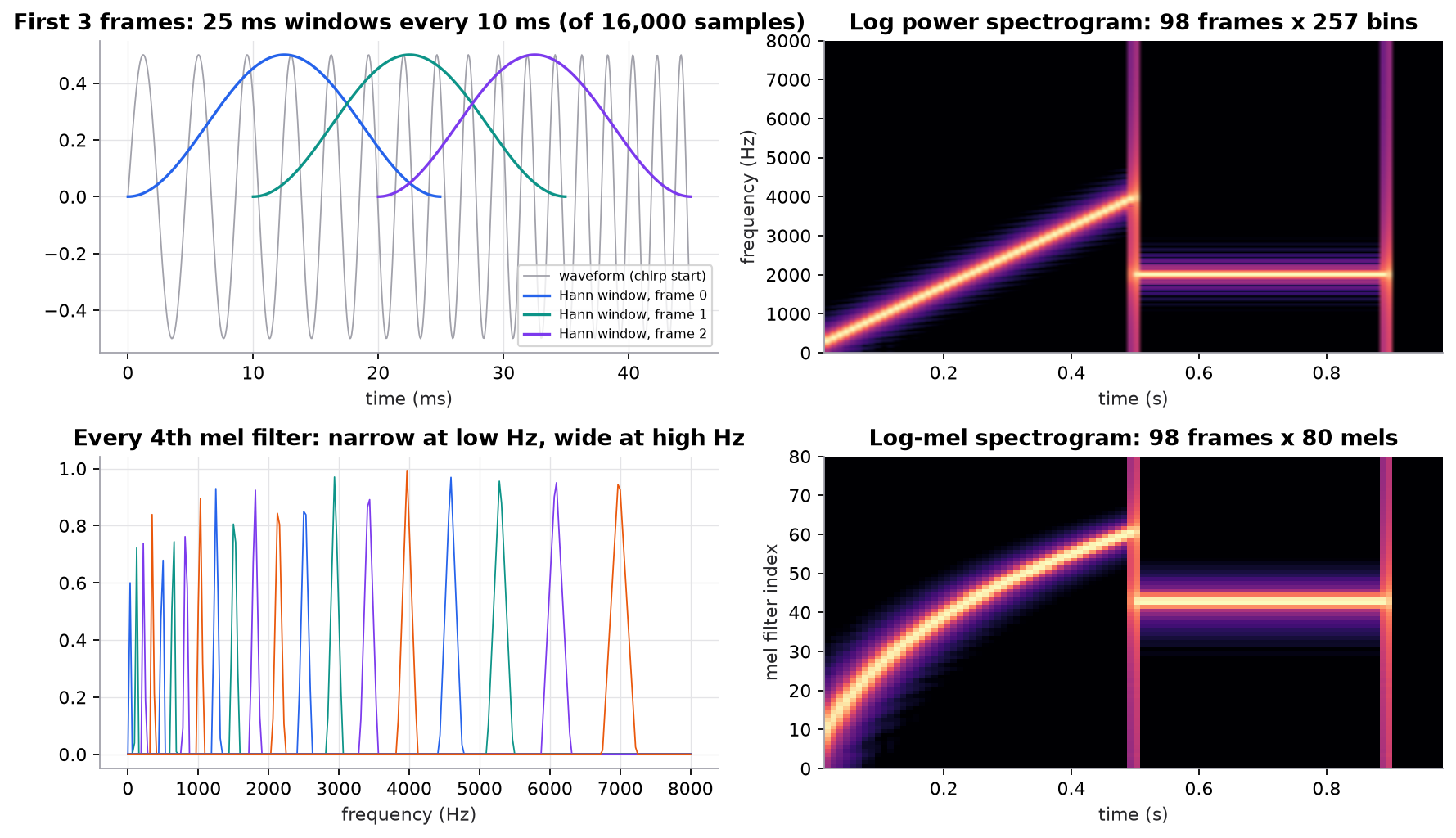
Synthetic signal: a chirp sweeping 200 to 4,000 Hz for 0.5 s, a 2 kHz tone until 0.9 s, then silence, sampled at 16 kHz.
Compare the two spectrograms. In hertz, the chirp is a straight line because its frequency rises linearly. In mels it bends: low frequencies get many mel bands, so the curve climbs fast at first, then high frequencies share fewer, wider bands, so it flattens. The vertical streaks at 0.5 s and 0.9 s are real: an abrupt change in a signal contains energy at all frequencies, which is also why clicks and plosives ("p", "t") look like vertical lines in speech spectrograms.
Try it (predict first, then edit mel_features.py):
- Set
WIN = 1600(100 ms). Predict what happens to the chirp line's thickness and to the sharpness of the 0.5 s transition. - Replace
hann(...)with a window of all ones (no tapering). Predict the change in the tone's spectrogram row. - Set
N_MELS = 128. Predict how many low filters cover just one FFT bin, and whether the chirp curve looks smoother. - Resample conceptually: change
SRto 8,000 while keeping the chirp to 4,000 Hz. Predict what happens to the top of the sweep. (Hint: the highest frequency a sampled signal can represent is half the sample rate.)
3. The math
Symbols
| Symbol | Meaning | Shape / unit |
|---|---|---|
| waveform sample | scalar, | |
| sample rate | Hz (samples per second) | |
| window length | samples | |
| hop length | samples | |
| number of frames | count | |
| window function | length | |
| FFT size (frame zero-padded to this) | samples | |
| power spectrogram | ||
| number of mel filters | count | |
| mel filterbank matrix | ||
| log-mel spectrogram |
Framing
Frame covers samples to .
Window and FFT
Hann window (periodic form, as in PyTorch and librosa): . Power spectrum of frame at bin :
Bin corresponds to frequency . Only bins up to are kept because a real signal's spectrum is symmetric.
Mel scale and filterbank
Place edges equally spaced in mel from to , convert back to hertz as . Filter is a triangle rising from to a peak of 1 at and falling to 0 at . For a bin at frequency :
Then the whole mel step is one matrix multiply and a log:
Worked example
Settings: , (1 s), , , , .
- Frames: . Frame shape .
- Bins: bins, spaced Hz. Power spectrogram shape .
- A 2 kHz tone lands at bin exactly.
- Mel range: mel. 82 edges from 0 to 2840.0 are mel apart.
- Where 2 kHz falls: mel. Edges 43 and 44 are at and mel, which convert to Hz and Hz.
- Weights for bin 64 (2,000 Hz): filter 42 (edges 42, 43, 44) is on its falling side: . Filter 43 (edges 43, 44, 45) is on its rising side: . The two weights sum to 1, because adjacent triangles overlap exactly.
- Shapes: is ; is ; MFCCs are .
- Filter widths: filter 0 spans 0 to 45 Hz, so with bins 31.25 Hz apart it contains a single FFT bin (31.25 Hz). Filter 79 spans 7,475 to 8,000 Hz (525 Hz). Equal steps in mel are very unequal in hertz.
Time versus frequency resolution. Bin spacing is , and each frame spans seconds. A longer window resolves nearby pitches but blurs fast events; a shorter one does the opposite. 25 ms / 10 ms is the speech compromise.
4. Implementation
Build it from scratch
All of it is NumPy. First, framing. Instead of a Python loop, build a index matrix: row is , and fancy indexing pulls every frame at once.
def frame(x, win=WIN, hop=HOP):
    n = 1 + (len(x) - win) // hop
    idx = np.arange(win)[None, :] + hop * np.arange(n)[:, None]           # [n_frames, win]
    return x[idx]
Predict: a 0.5 s clip at 16 kHz with the same window and hop gives how many frames?
Window and FFT. np.fft.rfft returns only the non-negative frequencies, and n=N_FFT zero-pads each 400-sample frame to 512.
def hann(n):
    return 0.5 - 0.5 * np.cos(2 * np.pi * np.arange(n) / n)              # periodic Hann (as torch/librosa)

def power_spectrum(frames, n_fft=N_FFT):
    spec = np.fft.rfft(frames * hann(frames.shape[1]), n=n_fft)           # [n_frames, n_fft//2 + 1]
    return np.abs(spec) ** 2
Predict: zero-padding to 512 makes the bins closer together (31.25 Hz instead of 40 Hz). Does it let you separate two tones 35 Hz apart? (No: padding interpolates the spectrum; true resolution is set by the 25 ms window.)
The mel conversion and the filterbank. Each row of fb is one triangle evaluated at every FFT bin's frequency.
def mel_filterbank(n_mels=N_MELS, n_fft=N_FFT, sr=SR, fmin=0.0, fmax=None):
    fmax = fmax or sr / 2
    edges_hz = mel_to_hz(np.linspace(hz_to_mel(fmin), hz_to_mel(fmax), n_mels + 2))  # equally spaced in mel
    bin_hz = np.arange(n_fft // 2 + 1) * sr / n_fft                                    # centre of each FFT bin
    fb = np.zeros((n_mels, len(bin_hz)))
    for m in range(n_mels):
        lo, c, hi = edges_hz[m], edges_hz[m + 1], edges_hz[m + 2]
        rise = (bin_hz - lo) / (c - lo)
        fall = (hi - bin_hz) / (hi - c)
        fb[m] = np.maximum(0, np.minimum(rise, fall))                     # triangle peaking at 1 at c
    return fb, edges_hz
Predict: what is the shape of fb for 80 mels and n_fft=512, and roughly how many nonzero entries does row 79 have? (Script: , 17.)
Log-mel is one matmul and a log; MFCC is a DCT-II written as another matmul with a cosine basis.
def log_mel(power, fb, eps=1e-10):
    return np.log10(np.maximum(power @ fb.T, eps))                      # [n_frames, n_mels]

def dct_ii(x, n_coeffs=13):
    N = x.shape[-1]
    n = np.arange(N)
    basis = np.cos(np.pi * np.arange(n_coeffs)[:, None] * (2 * n + 1) / (2 * N))   # [n_coeffs, N]
    return x @ basis.T
Predict: in a silent frame, what value does every log-mel entry take? (The floor: . That's why the floor value matters.)
Use the library
The same pipeline in one call each:
import torchaudio, librosa

mel = torchaudio.transforms.MelSpectrogram(sample_rate=16000, n_fft=400, win_length=400,
                                           hop_length=160, n_mels=80)(waveform)  # [channels, 80, frames]
log_mel = torch.log10(mel.clamp(min=1e-10))

S = librosa.feature.melspectrogram(y=y, sr=16000, n_fft=400, hop_length=160, n_mels=80)
mfcc = librosa.feature.mfcc(S=librosa.power_to_db(S), n_mfcc=13)
Note the conventions that differ from our script and from each other: libraries put time on the last axis (, not ); librosa's default mel scale is the Slaney variant (linear below 1 kHz) with area-normalized filters, while torchaudio's default is the HTK formula used here; power_to_db gives relative to a reference. Whisper computes 25 ms / 10 ms frames at 16 kHz, applies a mel filterbank (80 bands in most sizes, 128 in large-v3), takes , clips to 8 below the maximum, and rescales. If you feed a pretrained model, use its own feature extractor (for example the Hugging Face WhisperFeatureExtractor), never a re-implementation.
Run it
cd guide
uv run code/29-speech-and-audio/mel_features.py
Key output:
frames: 1 + (16000 - 400) // 160 = 98  -> shape (98, 400)
power spectrum shape (98, 257); bin spacing 31.25 Hz
frame 70 (t = 0.70 s): peak bin 64 -> 2000.0 Hz (true 2000 Hz)
filterbank shape (80, 257); filter 0 spans 0-45 Hz (45 Hz wide), filter 79 spans 7475-8000 Hz (525 Hz wide)
log-mel shape (98, 80); MFCC shape (98, 13)
  frame 25 (t = 0.263 s): mel 45, centre   2228 Hz, true   2195 Hz
silent frame 95: max log-mel -10.0 (floor log10(1e-10) = -10)
Full script: code/29-speech-and-audio/mel_features.py.
5. Engineering
Typical settings.
| Task | Sample rate | Window / hop | Features |
|---|---|---|---|
| Speech recognition | 16 kHz | 25 ms / 10 ms | 80 (sometimes 128) log-mels |
| Speech synthesis acoustic models | 22.05 or 24 kHz | about 46 ms / 11 ms | 80 to 100 log-mels |
| General audio classification | 16 to 32 kHz | 25 ms / 10 ms | 64 to 128 log-mels |
| Speaker verification, small devices | 16 kHz | 25 ms / 10 ms | log-mels or MFCC-13 to 40 |
Sample rate is part of the model. A model trained at 16 kHz fed 44.1 kHz audio sees every frequency scaled wrong. Resample at the input boundary, with a proper anti-aliasing filter (torchaudio.functional.resample, librosa.resample), and assert the rate in code.
Normalization must match training. Per-utterance mean/variance normalization, global statistics, or Whisper-style clipping and rescaling all produce different numbers. A mismatch can silently degrade accuracy. Ship the feature extractor with the model and test that features match on a golden file.
Padding and length. Whisper pads or trims every input to 30 s (3,000 frames). Streaming models need features computed incrementally with the same framing as offline. Zero-padding produces frames at the log floor; make sure the model saw the same during training, or pass an attention mask.
Compute. The front end is cheap next to the model (an FFT per 10 ms frame), but on small devices it matters: precompute the filterbank once, use real FFTs, and run in float32.
Augmentation. SpecAugment (masking random time and frequency bands of the log-mel) is a standard, cheap regularizer for speech models, applied to features during training only.
Common mistakes
- Feeding audio at the wrong sample rate, or resampling with naive decimation that aliases.
- Mixing natural log, , and decibels between training and serving.
- Transposing time and mel axes ( vs ) when moving between libraries.
- Too many mel filters for the FFT size, leaving low filters covering one or zero bins (librosa warns about empty filters).
- Re-implementing a pretrained model's feature extractor "close enough" instead of using its own.
- Forgetting the window, which smears every tone across neighbouring bins.
6. Knowledge check
Quiz: Spectrograms and mel features
A 2-second clip at 16 kHz is framed with a 400-sample window and a 160-sample hop (no padding). How many frames?
Practice exercise. A 3-second clip at 16 kHz uses a 25 ms window, 10 ms hop, , and 80 mels. Give the number of samples, frames, FFT bins, bin spacing in hertz, and the shapes of the power spectrogram, filterbank, and log-mel output.
Solution
Samples: . Window samples; hop .
Frames: .
Bins: , spacing Hz.
Power spectrogram ; filterbank ; log-mel .
(Libraries that center frames with padding give frames instead. Always check the center setting.)
Implementation challenge. Add delta features: for each log-mel frame , compute (edge-replicate the ends), then stack into a matrix. Check on the chirp that the delta is positive just above the chirp's current band and negative just below it.
Solution sketch
P = np.pad(S, ((1, 1), (0, 0)), mode="edge"), then delta = (P[2:] - P[:-2]) / 2, then np.hstack([S, delta]). As the chirp rises, the band just above it gets louder over time (positive delta) and the band it is leaving gets quieter (negative delta). Deltas were standard with MFCCs; neural models mostly learn temporal change themselves from stacked frames, but deltas still help small models.
Summary
- Speech front ends frame the waveform (25 ms window, 10 ms hop at 16 kHz), apply a Hann window, and take an FFT per frame to get a power spectrogram.
- The mel filterbank is an matrix of triangles equally spaced in mel; one matrix multiply turns 257 bins into 80 bands.
- Log compresses dynamic range; MFCCs add a DCT and keep about 13 coefficients, now mostly replaced by log-mels for neural models.
- Window length trades time resolution against frequency resolution.
- Sample rate, log base, normalization, axis order, and padding must match what the model was trained on.
Next: Speech recognition: CTC, transducers, and attention
Related: Convolutional networks · Recurrent networks · Transformer architecture
Go deeper, code-first (AI Engineering from Scratch): The Fourier Transform · Audio Fundamentals — Waveforms, Sampling, Fourier Transform · Audio Classification — From k-NN on MFCCs to AST and BEATs
Parts of this lesson are adapted from AI Engineering from Scratch by Rohit Ghumare (MIT license, notice): Spectrograms, Mel Scale & Audio Features.
Interview angle
Walk me through how raw audio becomes the input to a speech model.
Start with a mono waveform at the model's sample rate, usually 16 kHz. Cut it into overlapping frames, typically 25 milliseconds every 10 milliseconds, so 400 samples with a hop of 160. Multiply each frame by a Hann window so the edges taper to zero and the FFT doesn't smear energy. Take a real FFT and the squared magnitude, giving a power spectrum per frame. Multiply by a mel filterbank, a matrix of triangular filters equally spaced on the mel scale, which turns roughly 200 to 257 frequency bins into 80 bands, fine at low frequencies and coarse at high ones. Take the log, with a small floor, to compress dynamic range. Finally apply the same normalization the model was trained with. For a one-second clip that's a 98 by 80 matrix.
How do you choose the window length, and what does zero-padding the FFT buy you?
Window length sets the trade between time and frequency resolution. The true frequency resolution is about the sample rate divided by the window length, so 25 milliseconds gives roughly 40 hertz; a 100-millisecond window would resolve 10 hertz but blur anything faster than 100 milliseconds, like consonant onsets. Speech uses 25 milliseconds because speech is roughly stable over that span, and a 10-millisecond hop tracks how fast it changes. Music analysis often uses longer windows for pitch detail; drum or click detection uses shorter ones. Zero-padding the frame to a larger FFT size only interpolates the spectrum onto a finer grid. It makes peaks look smoother and can align bins with filter edges, but it cannot separate two tones the window itself can't resolve.
A speech model scores well offline but badly in production on the same kind of audio. Where do you look first?
The front end, before the model. First sample rate: production audio at 8 kHz telephony or 44.1 or 48 kHz from a browser fed into a 16 kHz model, or resampled without anti-aliasing. Second, the feature extractor itself: a re-implementation that uses natural log instead of log10, decibels instead of log power, a different mel scale variant, different normalization, or time and mel axes transposed. Third, padding and length: training clips padded to 30 seconds but production chunks of 2 seconds, or streaming code that frames differently at chunk boundaries. Fourth, channel and gain: stereo not downmixed, clipping, or very low levels. I'd dump features for the same file from the offline and production paths and diff them numerically, then add that golden-file comparison as a test.
How many feature frames does a 30-second clip produce at 16 kHz with a 10 ms hop, and what does that mean for a transformer encoder?
30 seconds at 100 frames per second is about 3,000 frames; with a 400-sample window and no centering it's 1 plus 479,600 over 160, which is 2,998. Self-attention cost grows with the square of sequence length, so 3,000 frames is expensive per layer. That's why speech encoders downsample early: Whisper's convolutional stem has a stride of 2, so the transformer sees 1,500 positions for 30 seconds; Conformer-style encoders often subsample by 4 or 8. With 80 mel bands, the input tensor is 80 by 3,000 per clip. Downsampling to 40 or 80 milliseconds per position still leaves enough resolution for characters or subword tokens.