Module 29: Speech and audio 45 min14 min quick readDeep learning
Speech recognition: CTC, transducers, and attention
Explain how speech recognizers align audio frames to text (CTC, RNN-T, attention encoder-decoder), decode CTC output greedily and with prefix beam search, compute the CTC loss with the forward algorithm, and measure word error rate.
Before this: Spectrograms and mel features, Recurrent networks, LSTMs, and GRUs, The transformer architecture
Quick read: the intuition, interactive visualization, summary, and interview questions. The math, implementation, engineering, and knowledge-check sections are hidden.
Mental model. A speech recognizer listens to 100 slices of sound per second but writes maybe 15 letters per second. Something has to decide which slices belong to which letter. CTC lets the model say "letter, letter, nothing, letter" for every slice and then squeezes out the repeats and the nothings. Transducers and attention models solve the same alignment problem in different ways.
You will learn to
- State the alignment problem in speech recognition and how CTC, RNN-T, and attention encoder-decoders each handle it.
- Decode CTC output with the collapse rule (greedy) and with prefix beam search, and explain why they can disagree.
- Compute the CTC probability of a transcript with the forward algorithm, and check it against brute force on a tiny example.
- Compute word error rate with edit distance, including the split into substitutions, deletions, and insertions.
- Choose an ASR architecture for offline, streaming, and on-device use.
Why it matters. Speech is an input to search, assistants, meeting notes, call analytics, and voice agents built on LLMs. Most teams use a pretrained recognizer, but choosing one, streaming it, and debugging it requires knowing how it aligns audio to text and how its errors are measured. CTC is also a general idea: any time a long input sequence must produce a shorter output sequence without known alignment (handwriting, sign language, DNA basecalling), CTC is a candidate.
1. Intuition
The alignment problem. After the front end, a clip is a sequence of feature frames, 100 per second. An encoder (convolutions, then a transformer or Conformer stack) turns them into hidden vectors, often downsampled to one per 40 to 80 ms. The transcript is a shorter sequence of tokens (characters or subwords). We don't know which frames produced which token, and a word can take 150 ms or 1.5 s. Training data has only (audio, transcript) pairs.
CTC (Connectionist Temporal Classification). Add a special blank token meaning "nothing new here". The model outputs a probability distribution over tokens-plus-blank at every frame, independently. Any frame-level path maps to text by a collapse rule: merge consecutive repeats, then delete blanks. So hh_e_ll_lloo becomes "hello": the blank between the two ll groups is what keeps the double letter. Training maximizes the total probability of all paths that collapse to the correct transcript. Decoding is fast because frames are independent. The cost is that independence: CTC can't model that "their" and "there" depend on the surrounding words, so it is often paired with an external language model at decode time.
RNN-T (transducer). Add a small prediction network that reads the tokens emitted so far, and a joint network that combines it with the current audio frame to predict "next token, or move to the next frame". Output now depends on previous outputs, an internal language model of sorts, while still processing audio left to right. That makes transducers the standard choice for streaming and on-device recognition. Training is heavier: the loss sums over a 2D lattice of (frame, token) positions. Token-and-duration transducers (TDT) also predict how many frames to skip, which speeds up decoding.
Attention encoder-decoder. The encoder reads all the audio; a transformer decoder generates tokens one at a time, cross-attending to any part of the encoder output. This is the same autoregressive generation as an LLM (see decoding); Whisper is the best-known example. It gives strong offline accuracy and handles punctuation, casing, and translation naturally. It doesn't stream without extra engineering, latency grows with output length, and like any autoregressive generator it can hallucinate: produce fluent text that wasn't said, especially on silence, music, or noise.
Measuring it: WER. Word error rate counts the minimum number of word substitutions, deletions, and insertions that turn the hypothesis into the reference, divided by the number of reference words. Lower is better, and it can exceed 1.0 because insertions are unbounded.
Key distinctionWER depends on text normalization. "Turn on the lights." and "turn on the lights" differ by casing and punctuation. Published comparisons apply a normalizer (lowercase, strip punctuation, standardize numbers and spellings) before computing WER. Comparing your system's raw WER to a published normalized WER is meaningless.
2. Visualization
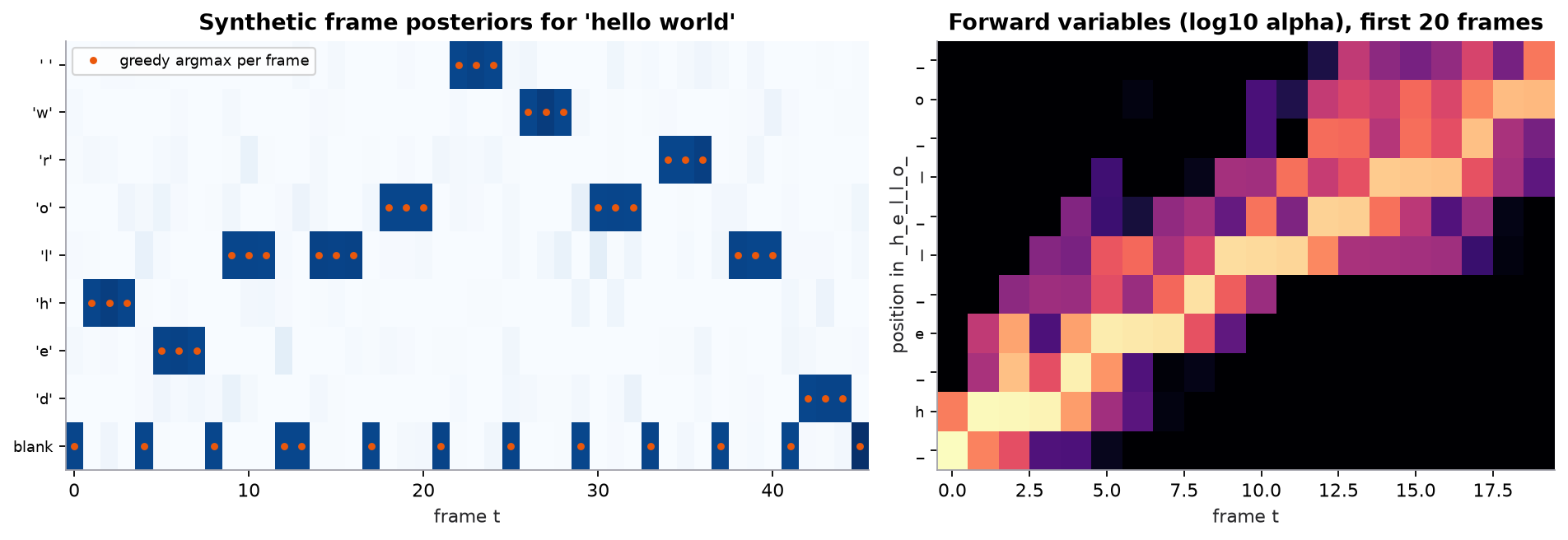
Synthetic posteriors (no audio): what an acoustic encoder might output for "hello world". Right: the forward algorithm's table, in log10, restricted to the first 20 frames.
On the left, the orange dots are greedy decoding: take the most likely token at each frame. Reading them in order gives _hhh_eee_lll_lll_ooo_ …, and the collapse rule turns that into "hello world". Note the blank between the two lll blocks: without it, the collapse would merge them into one l. On the right, each column is one frame and each row is a position in _h_e_l_l_o_. A bright cell means "a lot of probability flows through being at this label position at this frame". The diagonal band is the set of plausible alignments; the loss sums them all instead of picking one.
Try it (predict first, then edit ctc_asr.py):
- In
synthetic_posteriors, remove the line that inserts a blank between repeated letters. Predict the greedy output for "hello". - Lower
peakfrom 0.8 to 0.3. Predict whether greedy and beam search still agree, and what kinds of errors appear. - In the two-frame example, change the probabilities to , . Predict the greedy output and .
- Add the hypothesis "turn off the kitchen lights" to the WER list. Predict its WER and the S/D/I split.
3. The math
Symbols
| Symbol | Meaning | Shape / unit |
|---|---|---|
| encoder input (log-mel frames) | ||
| number of encoder output frames | count | |
| vocabulary size, not counting blank | count | |
| probability of token at frame (softmax output) | ||
| target transcript | length | |
| a frame-level path | length | |
| collapse map: merge repeats, delete blanks | path → text | |
| with blanks between and around tokens | length | |
| probability of all path prefixes up to frame ending at position of | ||
| substitutions, deletions, insertions, reference word count | counts |
CTC probability and loss
There are paths, far too many to enumerate. The forward algorithm sums them in time. With :
A path can stay at the same label, move one position forward, or skip one blank. The skip is allowed only when is not blank and : you can't jump over the blank between two identical letters, because that would merge them. It starts with , , and ends with (finish on the final blank or the final letter). A valid path needs , where is the number of adjacent repeated letters in , since each repeat needs a blank between.
Worked example: T = 3, vocabulary {blank, a}, target "a"
Frame probabilities (, ): , , . Extended target , .
Brute force. Of the paths, six collapse to "a":
__a ; _a_ ; _aa ; a__ ; aa_ ; aaa .
Sum . (___ gives "" and a_a gives "aa".)
Forward algorithm.
- : .
- , multiply by : ; ; .
- , probabilities for : ; ; .
- . ✓
- Loss .
Greedy is not the most probable transcript
Two frames, each with , . Greedy picks __, which collapses to "" with probability . But "a" collects three paths: aa + a_ + _a . The best path is not the best transcript. Prefix beam search fixes this by summing path probabilities per collapsed prefix.
Word error rate
Reference "turn on the kitchen lights" (), hypothesis "turn the kitchen light on": "on" deleted after "turn" (), "lights" → "light" (), "on" inserted at the end (). . The hypothesis "um so turn uh on the the kitchen lights please" contains every reference word but adds 5 insertions: .
4. Implementation
Build it from scratch
Start with the collapse rule and greedy decoding. prev tracks the last frame's token, so repeats merge, and blanks are dropped but still reset prev, which is what lets "ll" survive.
def collapse(ids):
    out, prev = [], None
    for i in ids:
        if i != prev and i != BLANK:
            out.append(i)
        prev = i
    return out

def greedy(probs):
    return "".join(VOCAB[i] for i in collapse(probs.argmax(1)))
Predict: what does collapse return for the path a a _ a b b?
The forward algorithm. Build the extended label sequence, then fill the table using stay, step, and skip.
def ctc_prob(probs, target):
    ext = [BLANK]
    for c in target:
        ext += [c, BLANK]                             # "ab" -> _ a _ b _ ; length 2U + 1
    S, T = len(ext), len(probs)
    alpha = np.zeros((T, S))
    alpha[0, 0] = probs[0, ext[0]]
    alpha[0, 1] = probs[0, ext[1]] if S > 1 else 0.0
    for t in range(1, T):
        for s in range(S):
            a = alpha[t - 1, s] + (alpha[t - 1, s - 1] if s >= 1 else 0.0)
            if s >= 2 and ext[s] != BLANK and ext[s] != ext[s - 2]:
                a += alpha[t - 1, s - 2]              # skip the blank between different letters
            alpha[t, s] = a * probs[t, ext[s]]
    return alpha[-1, -1] + (alpha[-1, -2] if S > 1 else 0.0), alpha
Predict: for the target "abb", which skip transitions are forbidden? (The jump from the first b over the blank to the second b.)
Real implementations work in log space (sums become log-sum-exp) because products of hundreds of probabilities underflow. The script checks the forward algorithm against brute-force enumeration on a random 6-frame case, so you can trust it.
Prefix beam search keeps, for each candidate text prefix, two probabilities: ending in blank and ending in a non-blank. The split is needed to decide whether the next identical letter extends the prefix or merges with it.
def prefix_beam(probs, beam=8):
    beams = {(): (1.0, 0.0)}                        # prefix -> (P ending in blank, P ending in non-blank)
    for p in probs:
        nxt = defaultdict(lambda: [0.0, 0.0])
        for prefix, (pb, pnb) in beams.items():
            nxt[prefix][0] += (pb + pnb) * p[BLANK]                    # emit blank: prefix unchanged
            for c in range(1, len(p)):
                if prefix and prefix[-1] == c:
                    nxt[prefix][1] += pnb * p[c]                       # repeat without blank: merges
                    nxt[prefix + (c,)][1] += pb * p[c]                 # blank in between: new letter
                else:
                    nxt[prefix + (c,)][1] += (pb + pnb) * p[c]
        beams = dict(sorted(nxt.items(), key=lambda kv: -sum(kv[1]))[:beam])
    best = max(beams.items(), key=lambda kv: sum(kv[1]))
    return "".join(VOCAB[i] for i in best[0]), sum(best[1])
Predict: on the two-frame example (, ), what does prefix_beam return? (Script: "a" with 0.64.) This is where an external language model plugs in: multiply each extension by when a word completes.
Word error rate is edit distance over words; the script also backtraces the table to count S, D, and I separately.
def wer(ref, hyp):
    r, h = ref.split(), hyp.split()
    d = np.zeros((len(r) + 1, len(h) + 1), dtype=int)
    d[:, 0], d[0, :] = np.arange(len(r) + 1), np.arange(len(h) + 1)
    for i in range(1, len(r) + 1):
        for j in range(1, len(h) + 1):
            d[i, j] = min(d[i - 1, j] + 1, d[i, j - 1] + 1, d[i - 1, j - 1] + (r[i - 1] != h[j - 1]))
Predict: "the cat sat" versus "the cat sat down". WER? (, one insertion.)
Use the library
Training with CTC in PyTorch is one loss call; inputs are log-probabilities shaped time-first.
import torch.nn.functional as F
loss = F.ctc_loss(log_probs,        # [T, batch, V+1], from log_softmax
                  targets,          # concatenated target ids
                  input_lengths, target_lengths, blank=0)
For inference, use a pretrained model:
from transformers import pipeline
asr = pipeline("automatic-speech-recognition", model="openai/whisper-large-v3-turbo")
print(asr("clip.wav", return_timestamps=True)["text"])   # long audio is chunked into 30 s windows
Other common choices: faster-whisper (CTranslate2 backend, faster CPU/GPU inference of Whisper models), NVIDIA NeMo (Parakeet and Canary families: transducer, CTC, and attention models; strong streaming support), and pyctcdecode for CTC beam search with an n-gram language model. Compute WER with jiwer after applying the same text normalizer to reference and hypothesis (Whisper ships an EnglishTextNormalizer). Check the Hugging Face Open ASR Leaderboard for current, normalized results on public test sets instead of quoting numbers from memory.
Run it
cd guide
uv run code/29-speech-and-audio/ctc_asr.py
Key output:
  forward algorithm P('a') = 0.770; brute force = 0.770; CTC loss = -ln P = 0.2614
  random check, T = 6, V = 4, target 'abb': forward 0.000370 vs brute force 0.000370
  P('a') = aa + a_ + _a = 0.16 + 0.24 + 0.24 = 0.64
  greedy -> ''; prefix beam -> 'a' with p = 0.64
  posteriors shape (46, 28) (frames x vocab)
  greedy: 'hello world'
  WER 0.60  S=1 D=1 I=1  'turn the kitchen light on'
  WER 1.00  S=0 D=0 I=5  'um so turn uh on the the kitchen lights please'
Full script: code/29-speech-and-audio/ctc_asr.py.
5. Engineering
Choosing an architecture.
| Need | Usual choice | Why |
|---|---|---|
| Best offline accuracy, punctuation, many languages | attention encoder-decoder (Whisper-style) or large transducer | full-context decoder, rich output |
| Live captions, voice agents, low latency | streaming transducer or chunked CTC | emits tokens as audio arrives |
| On-device, small footprint | small transducer or CTC with an n-gram LM | compact, no autoregressive decoder |
| Domain vocabulary (drug names, part numbers) | CTC/transducer with LM fusion or contextual biasing; or fine-tuning | boost rare words without retraining everything |
Long audio. Whisper-style models take 30 s windows. Split long audio with voice activity detection (VAD) at pauses, transcribe chunks (in parallel batches), and stitch with overlap. Splitting mid-word causes errors at the seams.
Hallucination. Autoregressive decoders can invent text on silence or music, or loop on a phrase. Mitigations: VAD to skip non-speech, compression-ratio and log-probability thresholds to reject degenerate outputs, temperature fallback, and not conditioning on the previous chunk's text when it's wrong.
Language and domain. Force the language when you know it; automatic language ID can misfire on short or noisy clips. Accented speech, telephone audio (8 kHz), far-field microphones, and overlapping speakers all raise WER sharply; evaluate on audio from your real channel, not just clean benchmarks.
Evaluation. Report WER on a held-out set from your domain with a fixed normalizer, plus a breakdown by speaker group, channel, and noise condition. For voice agents, also measure latency (time to first word, time to final transcript) and the effect of recognition errors on the downstream task, since the LLM may be robust to some errors and not others.
Privacy. Voice is biometric and often contains personal data. Decide what audio and transcripts you store, for how long, and whether processing can stay on device.
Common mistakes
- Comparing WER numbers computed with different normalizers or on different test sets.
- Feeding 44.1 kHz or 8 kHz audio to a 16 kHz model without resampling.
- Forgetting that CTC needs : downsampling the encoder too aggressively makes long or repetitive transcripts impossible to emit.
- Naive beam search that merges paths by collapsed text without tracking blank versus non-blank, which breaks double letters.
- Sending hours of audio to a 30-second-window model without chunking and VAD.
- Trusting confident-looking output on silence; attention decoders can produce fluent text from noise.
6. Knowledge check
Quiz: Speech recognition
Apply the CTC collapse rule (merge repeats, then delete blanks _) to the path cc_aa_t_t. What text results?
Practice exercise. Two frames, vocabulary {blank, a, b}, probabilities per frame : frame 1 , frame 2 . Compute , , , and , and give the greedy decode.
Solution
Paths of length 2:
"": __ .
"a": aa ; a_ ; _a . Total .
"b": bb ; b_ ; _b . Total .
"ab": ab . "ba": ba .
Check: . ✓
Greedy: frame 1 argmax is blank (0.5); frame 2 is a tie between blank and b (0.4). Breaking the tie toward blank gives ""; toward b gives "b". The most probable transcript is "b" (0.36), which beats "" (0.20) either way.
Implementation challenge. Convert ctc_prob to log space using np.logaddexp, and verify it matches the probability-space version on the "hello world" posteriors. Then compute the loss for a 200-frame synthetic utterance where the probability-space version underflows to 0.
Solution sketch
Store la = np.full((T, S), -np.inf), initialize with np.log of the first-frame probabilities, and replace each sum with np.logaddexp over the two or three predecessors, then add np.log(probs[t, ext[s]]). The final log-probability is np.logaddexp(la[-1, -1], la[-1, -2]). On "hello world" it should equal np.log of the original to about 1e-12. For long utterances, the product of hundreds of probabilities around 0.1 underflows float64 near , while the log version stays finite. This is exactly what F.ctc_loss does internally.
Summary
- Speech recognition must align many audio frames to fewer tokens without knowing the alignment.
- CTC predicts a token or blank per frame independently, collapses repeats and blanks, and trains on the sum over all valid paths, computed by the forward algorithm in O(T·S).
- Greedy CTC decoding picks the best path, not the best transcript; prefix beam search sums paths per prefix and is where language models plug in.
- Transducers add a prediction network for streaming with output dependencies; attention encoder-decoders like Whisper give strong offline quality but don't stream natively and can hallucinate.
- WER = (S + D + I) / N, computed after a fixed text normalization; it can exceed 1.
Next: Gradient clipping and mixed precision
Related: Spectrograms and mel features · Recurrent networks · Transformer architecture · LLM evaluation
Go deeper, code-first (AI Engineering from Scratch): Whisper — Architecture & Fine-Tuning · Text-to-Speech (TTS) — From Tacotron to F5 and Kokoro · Audio Evaluation — WER, MOS, UTMOS, MMAU, FAD, and the Open Leaderboards
Parts of this lesson are adapted from AI Engineering from Scratch by Rohit Ghumare (MIT license, notice): Speech Recognition (ASR) — CTC, RNN-T, Attention.
Interview angle
Explain CTC: what problem does it solve and how does the blank token work?
Speech gives many more frames than output characters, and training data has no frame-level alignment. CTC lets the network output a distribution over characters plus a blank at every frame, independently. A frame-level path maps to text by merging consecutive repeats and then removing blanks, so "hh_e_ll_lo" becomes "hello". The blank does two jobs: it fills frames where nothing new is said, and it separates genuine double letters, since "ll" without a blank between would merge into one "l". Training maximizes the total probability of all paths that collapse to the transcript, summed efficiently with a forward algorithm over the transcript interleaved with blanks, in time proportional to frames times label length. The main weakness is the conditional independence between frames, so CTC is often paired with a language model during beam search.
CTC, RNN-T, or attention encoder-decoder for a live captioning product? Why?
I'd lean toward a streaming transducer. Live captions need words on screen within a few hundred milliseconds, so the model must emit as audio arrives. A transducer processes audio left to right with limited lookahead, and its prediction network conditions on previous tokens, so it captures some language context that pure CTC lacks. CTC is the simpler, faster alternative: chunked encoders with CTC stream well and decode in parallel, and an n-gram or neural language model in beam search recovers much of the accuracy. An attention encoder-decoder like Whisper attends over a whole 30-second window and generates autoregressively, which gives great offline accuracy but needs chunking tricks and re-decoding to stream, adding latency and instability at chunk edges. I'd still measure: WER on our audio, latency to first and final word, and cost per hour.
Your Whisper-based transcription inserts sentences nobody said during long silences. How do you fix it?
That's decoder hallucination: an autoregressive model asked to produce text from near-silence generates fluent, plausible text, sometimes repeating earlier phrases or stock phrases from training data. First, stop feeding it silence: run voice activity detection and only transcribe speech regions. Second, use the decoder's own signals: reject or retry segments with a low average log-probability, a high no-speech probability, or a high compression ratio, which flags repetition loops. Third, check the decoding setup: conditioning on the previous segment's text can propagate a hallucination, so disable it after a bad segment, and use temperature fallback when greedy output looks degenerate. Then measure insertion rate separately from total WER on a test set with real silences, since insertions are exactly what this failure produces.
A reference has 20 words. The hypothesis has 2 substitutions, 1 deletion, and 3 insertions. What is the WER, and why can WER exceed 100 percent?
WER is substitutions plus deletions plus insertions over reference words: 2 plus 1 plus 3 is 6, over 20, so 0.30 or 30 percent. It can exceed 100 percent because insertions aren't bounded by the reference length. If the system outputs 25 extra words of hallucinated text on a 20-word reference while getting the 20 right, that's 25 over 20, or 125 percent. That's also why I look at the S, D, I breakdown rather than just the total: many deletions suggest VAD or chunking is cutting speech, many insertions suggest hallucination or noise being transcribed, and substitutions point at acoustic or vocabulary problems. All of it assumes reference and hypothesis went through the same normalizer.