Module 24: Applied ML in practice 45 min10 min quick readClassical ML
Feature engineering
Turn raw columns into model-ready features (scaling, log transforms, one-hot and target encoding, imputation with indicators, filter selection) without leaking the label.
Before this: Workflow, splits, and leakage, Probability and statistics
Quick read: the intuition, interactive visualization, summary, and interview questions. The math, implementation, engineering, and knowledge-check sections are hidden.
Mental model. A model only sees the columns you hand it. Feature engineering is translating the world into those columns: put numbers on comparable scales, turn categories into numbers without inventing an order, say "this was missing" out loud, and throw away columns that only add noise. Do it all with the training data alone, or you are handing the model the answers.
You will learn to
- Choose between standardization, min-max scaling, and a log transform for a numeric column, and say which models care.
- Encode categories with one-hot or smoothed target encoding, and compute a smoothed encoding by hand.
- Impute missing values and add a missing-indicator column.
- Explain why target encoding leaks and fix it with out-of-fold encoding.
- Filter features by variance, redundancy (correlation), and mutual information.
Why it matters. On tabular problems, better features usually beat a fancier model. A ratio like price per square foot or a "days since last purchase" column can do more than a week of tuning. Feature pipelines are also where most silent leakage bugs live, and interviewers know it.
1. Intuition
Think of each column as a question you ask about a row. The model can only combine the answers it gets.
Numbers need comparable scales. k-nearest neighbors, SVMs, k-means, and anything trained with gradient descent and a penalty compare or combine raw magnitudes. If square footage runs to 5,000 and age runs to 50, distance is almost all square footage. Standardization (subtract the mean, divide by the standard deviation) fixes this. Tree models split one column at a time on thresholds, so they don't care about scale.
Skewed numbers need compressing. Income, counts, and prices have long right tails. One huge value dominates a squared loss and squashes everyone else together. Taking log(1 + x) turns "50 times larger" into "about 3.9 larger", and turns multiplicative effects into additive ones a linear model can learn.
Categories need numbers without a fake order. Mapping red, green, blue to 0, 1, 2 tells a linear model that blue is "twice" green. One-hot encoding gives each category its own 0/1 column instead. When a column has thousands of values (zip code, merchant ID), one-hot explodes, so you can replace each category with the average label for that category: target encoding. It is powerful and the easiest way in this lesson to cheat by accident.
Missing is information. Fill a hole with the median so the model can run, but also add a was_missing column. A blank income field often means something (self-employed, refused to answer).
Fewer, better columns. A column that never varies carries nothing. Two columns that are copies of each other (square feet and square meters) double-count. A column unrelated to the label just gives the model more ways to overfit.
2. Visualization
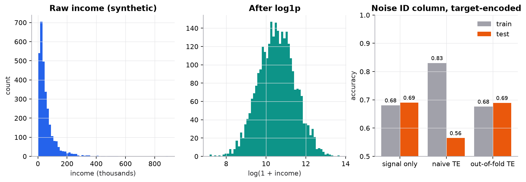
Synthetic data. Left and middle: a log transform turns a long-tailed income column into a roughly symmetric one. Right: an ID column with about two rows per ID is pure noise. Target-encoding it on the same rows the model trains on makes training accuracy jump from 0.68 to 0.83 while test accuracy falls to 0.56. Encoding it out of fold removes the fake signal.
Try it (predict first, then run code/24-applied-ml/feature_engineering.py):
- Change
n_idsfrom 1000 to 20 (about 100 rows per ID). Predict whether the gap between naive train and test accuracy grows or shrinks. - Raise the smoothing
min the leakage experiment from 1 to 50. Predict what happens to the naive encoder's weight on the ID feature. - In worked example 3, change the two
rurallabels to 0. Predict the new encoding before running. - Lower the correlation threshold in
drop_correlatedto 0.05. Which columns survive, and why is that a bad threshold?
3. The math
Symbols
| Symbol | Meaning | Shape |
|---|---|---|
| one numeric column over training rows | ||
| mean and (population) standard deviation of on training data | scalars | |
| standardized column | ||
| a category value | scalar | |
| number of training rows with category | scalar | |
| mean label of those rows | scalar | |
| global mean label | scalar | |
| smoothing strength (pseudo-count) | scalar | |
| mutual information between a feature and the label | scalar, nats |
Scaling and the log transform
, , , and come from training rows only and are reused, unchanged, on validation, test, and production rows.
Smoothed target encoding
This is a weighted average of the category's own mean and the global mean. A category seen twice is pulled hard toward ; a category seen 10,000 times keeps its own mean. It is the same idea as a Bayesian prior worth pseudo-rows.
Mutual information
It is 0 when the feature and label are independent and grows as knowing narrows down . Unlike correlation, it catches non-linear relationships. For a continuous feature we bin it first, so the estimate depends on the bins.
Worked example: standardization
, .
- Mean: .
- Squared deviations: , summing to .
- Variance: , so .
- .
Worked example: log1p
Incomes . The largest is times the smallest. After the transform: , , , . The gap between largest and smallest is . A ratio became a difference.
Worked example: smoothed target encoding
Ten training rows, . Labels: city has 6 rows with 1 positive, suburb 2 rows with 0 positives, rural 2 rows with 2 positives.
- Global mean: .
- City: , so . .
- Suburb: . .
- Rural: , . .
Rural's raw mean of 1.0 would scream "always positive" on two rows of evidence. Smoothing turns that into 0.42.
Worked example: median imputation with an indicator
. Present values sorted: . Median . Filled: ; indicator . The median ignores the 3000 outlier; the mean would have been .
Why target encoding leaks
If row is encoded with a table that includes row 's own label, the feature partly is the label. With and an ID seen twice, the encoding of row is : one third of it is the answer. The model learns to trust that column, and at test time, where the row's label is not in the table, the trust is misplaced. Out-of-fold encoding fixes it: split training rows into folds and encode each fold with a table fit on the other .
4. Implementation
Build it from scratch
Numeric transforms. The statistics are returned, not just the transformed column, because you must reuse the training mean and standard deviation on new rows.
def standardize(x):
    """z = (x - mean) / std, using population std. Fit on train, reuse mean/std on test."""
    x = np.asarray(x, dtype=float)
    mean, std = x.mean(), x.std()
    return (x - mean) / (std if std > 0 else 1.0), mean, std

def min_max(x):
    x = np.asarray(x, dtype=float)
    lo, hi = x.min(), x.max()
    return (x - lo) / (hi - lo) if hi > lo else np.zeros_like(x)

def log1p(x):
    """log(1 + x): compresses a right tail, keeps 0 at 0. Only for x > -1."""
    return np.log1p(np.asarray(x, dtype=float))
Predict: a test row has a value larger than the training max. What range does its min-max value fall in?
Smoothed target encoding. One pass per category: count, mean, then blend with the global mean.
def target_encode_fit(cats, y, m=10.0):
    """Smoothed mean: enc(c) = (n_c * mean_c + m * global_mean) / (n_c + m)."""
    y = np.asarray(y, dtype=float)
    g = y.mean()
    table = {}
    for c in set(cats):
        mask = np.array([v == c for v in cats])
        n_c, mean_c = mask.sum(), y[mask].mean()
        table[c] = (n_c * mean_c + m * g) / (n_c + m)
    return table, g
Predict: what does a category never seen in training get? (Look at how the callers use table.get(c, g).)
Out-of-fold encoding. Each training row is encoded by a table that never saw its label. Test rows use a table fit on all training rows.
def target_encode_oof(cats, y, m=10.0, k=5, seed=0):
    """Out-of-fold: each row is encoded with a table fit on the OTHER folds, so its own label never leaks in."""
    cats, y = np.asarray(cats), np.asarray(y, dtype=float)
    folds = np.random.default_rng(seed).permutation(len(y)) % k
    out = np.empty(len(y))
    for f in range(k):
        table, g = target_encode_fit(list(cats[folds != f]), y[folds != f], m)
        out[folds == f] = [table.get(c, g) for c in cats[folds == f]]
    return out
Predict: with about 2 rows per ID and , how often does a row's ID appear in the other folds at all? What value does it get when it doesn't?
Imputation with an indicator.
def impute_median_with_indicator(x):
    """Fill NaN with the median of present values, and return a was_missing column."""
    x = np.asarray(x, dtype=float)
    miss = np.isnan(x)
    med = np.median(x[~miss])
    return np.where(miss, med, x), miss.astype(int), med
Predict: if missingness is random, will the model put any weight on the indicator?
Filter selection. Mutual information on a binned feature, and a greedy redundancy filter.
def mutual_information(feature, target, n_bins=10):
    """MI between an equal-width-binned feature and a discrete target, in nats."""
    f = np.asarray(feature, dtype=float)
    t = np.asarray(target)
    edges = np.linspace(f.min(), f.max(), n_bins + 1)
    b = np.clip(np.digitize(f, edges[1:-1]), 0, n_bins - 1)
    mi = 0.0
    for bi in np.unique(b):
        for ti in np.unique(t):
            p_joint = np.mean((b == bi) & (t == ti))
            if p_joint > 0:
                mi += p_joint * math.log(p_joint / (np.mean(b == bi) * np.mean(t == ti)))
    return mi

def drop_correlated(X, threshold=0.9):
    """Greedy: keep column i, drop any later column j with |r_ij| >= threshold."""
    r = np.corrcoef(X, rowvar=False)
    keep = []
    for j in range(X.shape[1]):
        if all(abs(r[i, j]) < threshold for i in keep):
            keep.append(j)
    return keep
Predict: the label is with symmetric around 0. Which is near zero, the correlation or the mutual information?
Use the library
scikit-learn composes the same steps into one object that is fit on training data only, which is the main protection against leakage. TargetEncoder (scikit-learn 1.3+) cross-fits automatically: fit_transform encodes training rows out of fold, while transform on new rows uses the full table.
from sklearn.compose import ColumnTransformer
from sklearn.impute import SimpleImputer
from sklearn.pipeline import Pipeline
from sklearn.preprocessing import OneHotEncoder, StandardScaler, TargetEncoder

pre = ColumnTransformer([
    ("num", Pipeline([("impute", SimpleImputer(strategy="median", add_indicator=True)),
                      ("scale", StandardScaler())]), num_cols),
    ("ids", TargetEncoder(target_type="binary"), high_card_cols),
    ("cat", OneHotEncoder(handle_unknown="ignore"), low_card_cols),
])
model = Pipeline([("pre", pre), ("clf", LogisticRegression())]).fit(X_train, y_train)
Put the whole pipeline inside cross_val_score or a search, never a pre-transformed matrix. Other tools: VarianceThreshold, mutual_info_classif (a k-NN estimator, no binning), SelectFromModel with an L1 model, and RFECV. Gradient-boosted tree libraries (LightGBM, CatBoost) handle categories natively; CatBoost's ordered target statistics are another out-of-fold scheme.
Run it
From guide/:
uv run code/24-applied-ml/feature_engineering.pyKey output:
mean = 5.0, std = 2.0, z = [-1.5, -0.5, -0.5, -0.5, 0.0, 0.0, 1.0, 2.0]
  rural   n=2  raw mean=1.00  encoded=0.4167
  signal only     train acc = 0.681   test acc = 0.691
  naive TE        train acc = 0.831   test acc = 0.565
  out-of-fold TE  train acc = 0.676   test acc = 0.690
  sqft_m2      var(min-max) = 0.0810   MI = 0.4806 nats   drop: |r| >= 0.9 with an earlier column
  constant_ish var(min-max) = 0.0040   MI = 0.0000 nats   drop: variance < 0.01
  pipeline test acc = 0.689
The naive encoder's weight on the noise ID column is +8.06; out of fold it is +0.66.
5. Engineering
Which models need what. Distance and gradient-based models (k-NN, SVM, k-means, linear and logistic regression with a penalty, neural networks) need scaling. Trees and tree ensembles don't, and handle monotonic transforms such as log for free, but still benefit from ratios and differences they cannot easily build from one-column splits.
Domain features beat generic ones. Ratios (debt to income), differences (days between signup and first purchase), aggregates over a window (orders in the last 30 days), and counts usually carry more signal than any automatic polynomial expansion. Polynomial features grow as for degree 2 and overfit quickly.
Encoding by cardinality. Under about 20 values: one-hot. Hundreds to millions: target encoding (cross-fitted), frequency encoding, hashing, or learned embeddings. Always plan for unseen categories at serving time (handle_unknown="ignore", fall back to the global mean).
Training-serving skew. The same code must compute features offline and online, with the same fitted statistics. Save the fitted pipeline as one artifact. Time-windowed aggregates must use only data available at prediction time: see time series. A feature store exists to solve exactly this.
Selection cost. Filters (variance, correlation, mutual information) are cheap and model-agnostic but judge one feature at a time. Wrappers (recursive elimination) and embedded methods (L1) account for interactions but cost model fits. Any selection that looks at labels must happen inside cross-validation.
Watch outFailure modes. Fitting the scaler or encoder on all data before splitting; target encoding without cross-fitting; features computed with future information (a "total purchases" column that includes purchases after the prediction date); one-hot columns that differ between train and serving because a category appeared or vanished.
Common mistakes
- Calling
fit_transformon the test set instead oftransform. - Label-encoding nominal categories (red=0, green=1, blue=2) for a linear model.
- Applying
logto a column with zeros or negatives (uselog1p, or a signed transform). - Imputing without an indicator when missingness is informative.
- Dropping a feature because its correlation with the label is low, when the relationship is non-linear.
- Selecting features on the full dataset, then cross-validating the selected set (optimistic scores).
6. Knowledge check
Quiz: Feature engineering
Why is feature engineering often more impactful than choosing a fancier algorithm on tabular data?
Practice exercise. A merchant ID column has three values in training: A (8 rows, 2 positives), B (2 rows, 2 positives), C (10 rows, 1 positive). Compute the smoothed target encoding of each with , and say what an unseen merchant D gets.
Solution
Global mean , so .
- A: .
- B: . Raw mean 1.0, pulled strongly toward 0.25 because it has only 2 rows.
- C: .
- D (unseen): the global mean, 0.25.
Implementation challenge. Add a robust_scale(x) that uses the median and the interquartile range instead of the mean and standard deviation. Feed it [1, 2, 3, 4, 100] and compare with standardize.
Solution
def robust_scale(x):
    x = np.asarray(x, dtype=float)
    q1, med, q3 = np.percentile(x, [25, 50, 75])
    return (x - med) / (q3 - q1 if q3 > q1 else 1.0)
Median 3, Q1 2, Q3 4, IQR 2: [-1, -0.5, 0, 0.5, 48.5]. The four normal points stay spread out. standardize gives mean 22 and std about 39.0, so the four normal points all land between -0.54 and -0.46, squashed together by one outlier. scikit-learn's RobustScaler does the same.
Summary
- Scale numeric features for distance and gradient-based models; trees don't need it. Fit the statistics on training rows only.
- Use
log1pon long-tailed, non-negative columns: ratios become differences. - One-hot low-cardinality categories; target-encode high-cardinality ones with smoothing and out-of-fold fitting.
- Impute and add a missing indicator; missingness is often a signal.
- Filter by variance, redundancy, and mutual information, inside cross-validation.
Next: Imbalanced data
Related: The ML workflow · Text to vectors (TF-IDF) · Regularization · Hyperparameter tuning
Go deeper, code-first (AI Engineering from Scratch): Feature Selection
Parts of this lesson are adapted from AI Engineering from Scratch by Rohit Ghumare (MIT license, notice): Feature Engineering & Selection.
Interview angle
What is target encoding, and why can it leak even when you only use training data?
Target encoding replaces each category with the average label for that category, usually smoothed toward the global mean: (n_c times the category mean plus m times the global mean) divided by (n_c plus m). It turns a column with thousands of values into one numeric column. The leak is subtle: if a training row is encoded with a table that includes its own label, the feature contains part of the answer. For a rare category it can be mostly the answer. The model learns to trust the column, training accuracy jumps, and on new rows, whose labels aren't in the table, the trust is wrong. In the course's synthetic experiment a pure-noise ID column pushed train accuracy from 0.68 to 0.83 while test fell from 0.69 to 0.56. The fix is cross-fitting: encode each fold with a table built from the other folds. scikit-learn's TargetEncoder does this in fit_transform; CatBoost uses ordered statistics.
When do you scale features, and which scaler do you pick?
Scale when the model compares or combines raw magnitudes: k-NN, SVMs, k-means, PCA, regularized linear models, and neural networks. Without it, the column with the largest units dominates distances and the penalty treats coefficients unfairly. Tree models split one feature at a time on thresholds, so scaling changes nothing for them. Standardization (subtract mean, divide by standard deviation) is the default. Min-max scaling to 0 to 1 suits bounded inputs such as pixel intensities but is ruined by one outlier, and new values can fall outside the range. Robust scaling with the median and interquartile range resists outliers. For long right tails, apply log1p first, because no linear scaler fixes skew. In every case, fit on the training split, save the statistics with the model, and reuse them at serving time. Fitting on all data before splitting leaks test-set information into training.
Your model scores 0.95 AUC offline and 0.70 in production. How would you check whether features are to blame?
I'd look for leakage first, then skew. Leakage: rank features by importance and ask of each top feature whether it is truly known at prediction time. Classic culprits are aggregates computed over the whole history (including the future), target encodings fit without cross-fitting, IDs that correlate with the label because of how data was collected, and preprocessing fit on the full dataset. A quick test is to retrain with a strict time-based split; if the offline score drops toward 0.70, the original split was leaking. Skew: log the feature values the production model actually received and compare their distributions with training. Different null rates, unit changes, unseen categories mapped to zeros, or a window computed differently online all show up there. The durable fix is one shared feature definition used offline and online, and the whole pipeline saved as one artifact.
A category seen 2 times has 2 positives; the global positive rate is 0.3. What is its target encoding with smoothing m = 10, and why smooth at all?
The smoothed encoding is (n_c times the category mean plus m times the global mean) divided by (n_c plus m). Here that is (2 times 1.0 plus 10 times 0.3) divided by (2 plus 10), which is (2 plus 3) over 12, or 5 over 12, about 0.417. Without smoothing the encoding would be 1.0, a claim of certainty from two rows. Smoothing is a prior worth m pseudo-rows at the global rate: categories with little data stay near 0.3, while a category with 10,000 rows keeps essentially its own mean. That shrinks noise from rare categories, which is where overfitting and leakage hurt most. m is a hyperparameter; values from a few to a few dozen are common, and you can tune it with cross-validation. scikit-learn's TargetEncoder picks the smoothing automatically from the variances by default.