Module 24: Applied ML in practice 45 min11 min quick readClassical ML
Hyperparameter tuning
Search hyperparameters efficiently with random search, successive halving, and Bayesian optimization, on log scales, and report an honest score with nested cross-validation.
Before this: Overfitting and the bias-variance trade-off, Workflow, splits, and leakage
Quick read: the intuition, interactive visualization, summary, and interview questions. The math, implementation, engineering, and knowledge-check sections are hidden.
Mental model. Tuning is a search for the best settings on a map you can only see one expensive point at a time. Grid search walks a fixed checkerboard. Random search throws darts, which hits more distinct values of the knobs that matter. Successive halving gives many darts a quick look and spends real compute only on the promising ones. Bayesian optimization draws a rough map from the darts so far and aims the next one where it looks best or least known.
You will learn to
- Separate parameters (learned) from hyperparameters (chosen), and pick log-scale ranges for scale-like knobs.
- Explain, with numbers, why random search beats grid search when only a few hyperparameters matter.
- Compute the cost of successive halving and say when early elimination can mislead.
- Build a Gaussian-process surrogate with expected improvement and say when it helps.
- Use nested cross-validation to report a score that the search has not overfit.
Why it matters. Most models ship with defaults that are close but not best, and tuning is where compute budgets quietly disappear. Interviewers ask about it constantly because it tests three things at once: search strategy, cost reasoning, and whether you understand that a tuned validation score is optimistic.
1. Intuition
A parameter is learned from data: a weight, a split threshold. A hyperparameter is set before training and controls how learning happens: learning rate, tree depth, regularization strength, number of neighbors.
Not every knob matters. On a given problem, one or two hyperparameters usually drive most of the score (for gradient boosting, the learning rate and number of trees; for an RBF SVM, C and gamma). Grid search spends most of its budget on the knobs that don't matter. A 3 by 3 grid tries 9 configurations but only 3 distinct learning rates. Nine random trials try 9 distinct learning rates.
Search on the right scale. A learning rate of 0.001 versus 0.01 is as big a change as 0.01 versus 0.1. Sample such knobs uniformly in the exponent (log-uniform), not uniformly in value, or almost every sample lands between 0.1 and 1.
Kill bad runs early. A configuration that is clearly bad after one epoch is rarely great after a hundred. Successive halving trains many configurations briefly, keeps the best third, trains those longer, and repeats. Hyperband runs several of these brackets with different starting budgets to hedge against "slow starters".
Learn from past trials. Random search ignores results. Bayesian optimization fits a cheap model (the surrogate) of score versus settings, with uncertainty, and picks the next trial with an acquisition function that trades exploiting good regions against exploring unknown ones.
The tuned score is optimistic. If you try 100 settings and report the best validation score, part of that score is luck on that validation set. To report performance, wrap the whole search inside an outer cross-validation loop.
2. Visualization
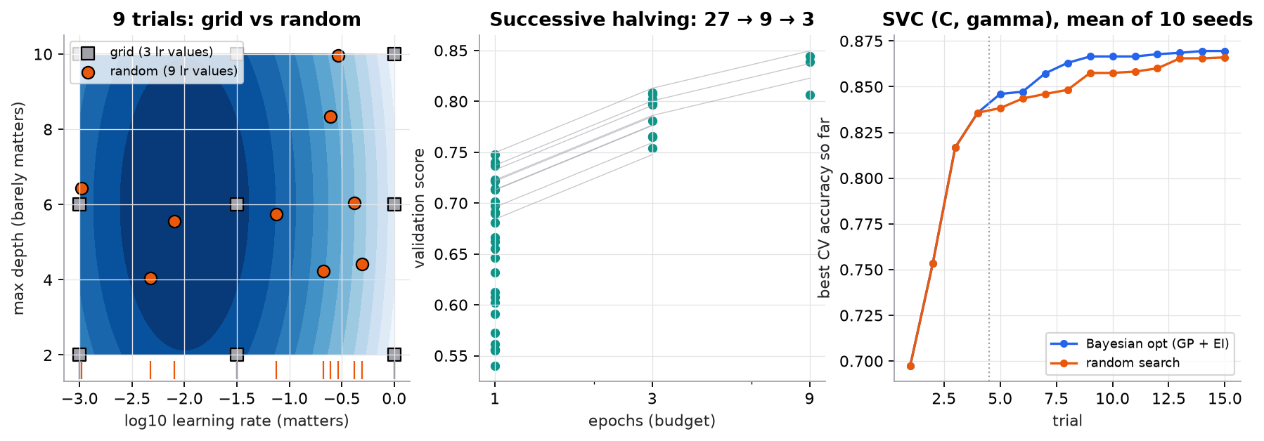
Left and middle use a synthetic score surface and synthetic learning curves; right tunes a real SVC on a synthetic dataset with 5-fold cross-validation. The grid's three learning rates all miss the optimum at 0.01; random search's nine distinct values get closer.
Try it (predict first, then run code/24-applied-ml/hyperparameter_tuning.py):
- Move the optimum in
score_surfacefromlog_lr + 2.0tolog_lr + 1.5(lr = 0.0316, exactly a grid value). Predict how often random search now beats the grid. - Change successive halving's
etafrom 3 to 2. Predict the number of rounds and the total cost in epochs. - Make the learning curves cross: give configs with a high
finala slower start. Predict whether successive halving still finds the best one. - Raise
budgetin Part 3 from 15 to 40. Predict whether the gap between Bayesian optimization and random search grows or shrinks.
3. The math
Symbols
| Symbol | Meaning | Shape |
|---|---|---|
| one hyperparameter configuration | ||
| validation score of a model trained with (expensive, noisy) | scalar | |
| number of trials | scalar | |
| fraction of the search space that is "good enough" | scalar | |
| successive-halving reduction factor | scalar | |
| surrogate's predicted mean and standard deviation of | scalars | |
| best score observed so far | scalar | |
| small exploration margin in expected improvement | scalar | |
| standard normal CDF and density | functions |
Random search: chance of a good trial
If a fraction of the space is good enough, each random trial misses it with probability , independently, so
Successive halving cost
Start configurations at budget ; each round keeps the top and multiplies the budget by . Round costs , the same every round. With rounds, total cost is .
Expected improvement (maximizing)
The first term rewards a high predicted score (exploit). The second rewards uncertainty (explore). A Gaussian process provides and ; Optuna's default TPE sampler models good and bad regions with density estimators instead, but the trade-off is the same.
Worked example: grid versus random on the synthetic surface
The score is , best at lr , depth 6.
- The 3 by 3 grid uses and depth .
- Its best point is , depth 6: .
- Random search with the same 9 trials averages over 2,000 seeds and beats the grid in 88% of them, because it tries 9 learning rates instead of 3.
Worked example: how many random trials
Take (the top 5% of the space):
- : .
- : .
- : .
This is the source of the "60 random trials" rule of thumb. It is about landing in the top 5% of the space you defined; a bad range is still bad.
Worked example: successive halving cost
, epoch, , maximum 9 epochs:
- Round 0: 27 configs × 1 epoch = 27 epochs. Keep .
- Round 1: 9 configs × 3 epochs = 27 epochs. Keep 3.
- Round 2: 3 configs × 9 epochs = 27 epochs. Pick the best.
- Total epochs, versus to train every config fully: one third of the cost. In the script the winner is the true best (final score 0.899), because these synthetic curves never cross.
Worked example: expected improvement at two candidates
Best so far , , so the bar is .
- Candidate A (unexplored): , . . , . .
- Candidate B (near known good points): , . . , . .
B wins here, but only narrowly: A's value comes entirely from uncertainty. Doubling A's to gives , and A would win.
4. Implementation
Build it from scratch
Part 1: grid and random points. Learning rate is searched in , from to .
def grid_points(n_per_axis):
    lrs = np.linspace(-3, 0, n_per_axis)            # log10 learning rate in [1e-3, 1]
    depths = np.linspace(2, 10, n_per_axis)
    return np.array([(a, b) for a in lrs for b in depths])

def random_points(n, rng):
    return np.c_[rng.uniform(-3, 0, n), rng.uniform(2, 10, n)]
Predict: with 4 hyperparameters and 3 values each, how many grid points, and how many distinct values of the one important knob?
Part 2: successive halving. Every round costs the same; the budget per survivor grows as the survivors shrink.
def successive_halving(finals, min_budget=1, max_budget=9, eta=3, rng=None):
    """Run all configs at min_budget, keep the top 1/eta, multiply budget by eta, until max_budget."""
    alive = np.arange(len(finals))
    budget, cost, rounds = min_budget, 0, []
    while True:
        scores = np.array([curve(finals[i], budget) + rng.normal(0, 0.01) for i in alive])
        cost += budget * len(alive)
        rounds.append((budget, alive.copy(), scores))
        if budget >= max_budget:
            return alive[np.argmax(scores)], cost, rounds
        alive = alive[np.argsort(-scores)[: max(1, len(alive) // eta)]]
        budget *= eta
Predict: if the noise 0.01 grew to 0.05, what kind of configuration would most often be wrongly cut in round 0?
Part 3a: the surrogate. A Gaussian process predicts a mean and an uncertainty at any point from the trials so far. Points close (in kernel distance) to observed trials get confident predictions; far points revert to the average with high uncertainty.
def rbf(a, b, length=0.8):
    """Squared-exponential kernel between rows of a [n, d] and b [m, d]. Returns [n, m]."""
    d2 = ((a[:, None, :] - b[None, :, :]) ** 2).sum(-1)
    return np.exp(-0.5 * d2 / length**2)

def gp_posterior(x_obs, y_obs, x_new, noise=0.05):
    """GP with zero mean on standardized y. Returns predictive mean and std at x_new."""
    mu_y, sd_y = y_obs.mean(), y_obs.std() + 1e-9
    y = (y_obs - mu_y) / sd_y
    K = rbf(x_obs, x_obs) + noise * np.eye(len(x_obs))
    Ks = rbf(x_obs, x_new)
    alpha = np.linalg.solve(K, y)
    mean = Ks.T @ alpha
    var = 1.0 - np.sum(Ks * np.linalg.solve(K, Ks), axis=0)
    return mean * sd_y + mu_y, np.sqrt(np.clip(var, 1e-12, None)) * sd_y
Predict: what happens to at a point exactly on an observed trial as noise goes to 0?
Part 3b: acquisition and the loop. Score 2,000 random candidates with EI and evaluate the best.
def expected_improvement(mean, std, best, xi=0.01):
    """EI = (mu - best - xi) * Phi(z) + sigma * phi(z), with z = (mu - best - xi) / sigma (maximizing)."""
    imp = mean - best - xi
    z = imp / std
    Phi = 0.5 * (1 + np.vectorize(math.erf)(z / math.sqrt(2)))
    phi = np.exp(-0.5 * z**2) / math.sqrt(2 * math.pi)
    return imp * Phi + std * phi

def bayes_opt(objective, lo, hi, n_init, n_iter, rng):
    """lo, hi: arrays [d] bounding the (log-scale) box. Candidates: 2,000 random points per step."""
    xs = list(rng.uniform(lo, hi, (n_init, len(lo))))
    ys = [objective(x) for x in xs]
    for _ in range(n_iter):
        cand = rng.uniform(lo, hi, (2000, len(lo)))
        mean, std = gp_posterior(np.array(xs), np.array(ys), cand)
        x_next = cand[np.argmax(expected_improvement(mean, std, max(ys)))]
        xs.append(x_next)
        ys.append(objective(x_next))
    return np.array(xs), np.array(ys)
Predict: with set to 0.2 (larger than any plausible gain), which term of EI dominates, and how will the search behave?
Use the library
from scipy.stats import loguniform
from sklearn.model_selection import RandomizedSearchCV, cross_val_score

space = {"C": loguniform(1e-2, 1e3), "gamma": loguniform(1e-4, 1e1)}
search = RandomizedSearchCV(SVC(), space, n_iter=30, cv=cv, random_state=0)
nested = cross_val_score(search, X, y, cv=outer_cv) # the honest estimateGridSearchCV/RandomizedSearchCVrefit the best configuration on all data passed tofit. Pass aPipelineso preprocessing is refit inside every fold.HalvingGridSearchCV/HalvingRandomSearchCVimplement successive halving. They are still experimental in scikit-learn and needfrom sklearn.experimental import enable_halving_search_cvfirst.- Optuna is the common standalone choice: define-by-run search spaces, TPE sampling by default, and pruners (median, successive halving, Hyperband) that stop trials using intermediate scores you report. Ray Tune distributes trials across machines.
- For gradient boosting, don't tune the number of trees: set it high and use early stopping on a validation set.
Run it
From guide/:
uv run code/24-applied-ml/hyperparameter_tuning.pyKey output:
grid best score = 0.8800
random best score, mean over 2000 seeds = 0.8903  (beats grid in 88% of seeds)
P(at least one of 60 random trials lands in the top 5% of the space) = 1 - 0.95^60 = 0.954
total cost = 81 epochs vs 243 to train all 27 for 9 epochs
  after  4 trials: Bayesian opt best = 0.8357   random best = 0.8357
  after  8 trials: Bayesian opt best = 0.8630   random best = 0.8482
  after 15 trials: Bayesian opt best = 0.8695   random best = 0.8660
RandomizedSearchCV best inner-CV score = 0.8825  params = C=7.1, gamma=0.0156
nested CV score = 0.8475 +/- 0.0406  (outer folds never seen by the search)
Two honest readings. Bayesian optimization helps most in the middle of a small budget; by trial 15 on this easy 2-D problem, random search has nearly caught up. And the search's own best score (0.8825) is higher than the nested estimate (0.8475): the gap is the optimism from picking the best of 30 on the same folds, plus fold-to-fold noise (the outer standard deviation is 0.04).
5. Engineering
Order of attack. Start from library defaults. Run a coarse random search (20 to 50 trials) over wide log ranges with early stopping. Look at which knobs correlate with score, narrow the ranges, then spend the rest on Bayesian optimization or a focused random search. Retrain the chosen configuration on all training data.
What to tune first. Learning rate (always), regularization strength, then capacity (depth, width, leaves). For boosting, number of trees comes from early stopping. Batch size, activation choice, and max features usually matter less within sensible ranges.
Compute. Cost is trials × folds × fit time. 50 trials × 5 folds × 2 minutes is over 8 hours; nested CV with 5 outer folds multiplies that by 5. Parallelize trials (random search is embarrassingly parallel; Bayesian optimization needs batch or asynchronous variants), tune on a subsample, and prune.
Reproducibility. Log every trial (config, seed, score, time) and fix seeds. Re-run the top few configs with different seeds before trusting a small gap; differences smaller than the seed-to-seed spread are noise.
Which metric. Tune on the metric you will ship with (AUPRC or recall at a fixed precision for imbalanced data, not accuracy). For time series, use time-ordered folds (time series).
Watch outFailure modes. Tuning on the test set (then it is no longer a test set). Linear sampling of scale-like knobs. A best value sitting on the edge of the range, meaning the range is wrong. Successive halving discarding slow starters (models with small learning rates often look worst early). Preprocessing fit outside the CV loop, which leaks into every trial.
Common mistakes
- Reporting
best_score_as the model's expected performance. - Grid search over 5 or more hyperparameters.
- Tuning the number of boosting rounds or epochs instead of using early stopping.
- Comparing two configurations from a single run each, with no seed variance.
- Forgetting that
refit=Trueretrains on all data, sobest_estimator_was not the model scored in CV.
6. Knowledge check
Quiz: Hyperparameter tuning
Which of these is a hyperparameter rather than a parameter?
Practice exercise. You run successive halving with configurations, , a starting budget of 1 epoch, and a maximum of 27 epochs. How many rounds are there, how many configurations reach 27 epochs, and what is the total cost compared with training all 81 for 27 epochs?
Solution
Budgets 1, 3, 9, 27: four rounds. Survivors 81, 27, 9, 3, so 3 configurations reach 27 epochs. Each round costs epochs, so the total is epochs. Training everything fully costs epochs, so successive halving uses about 15% of the compute.
Implementation challenge. Add an upper-confidence-bound acquisition, , and compare it with EI in the script for and .
Solution
def ucb(mean, std, kappa=2.0):
    return mean + kappa * std
In bayes_opt, replace the expected_improvement(...) call with ucb(mean, std, kappa). Small exploits: it refines around the best point found and can get stuck on a local bump. Large explores: it samples corners with high uncertainty and improves more slowly at first. Expect to trail early and catch up later on this smooth 2-D surface; average over several seeds before concluding anything, since single runs differ by more than the gap.
Summary
- Hyperparameters are chosen, not learned; search scale-like ones on a log scale.
- Random search beats grid search when only a few knobs matter: same budget, more distinct values of the important ones. .
- Successive halving and Hyperband spend equal compute per round and cut total cost several-fold, at the risk of discarding slow starters.
- Bayesian optimization (GP or TPE surrogate plus an acquisition such as EI) helps most when trials are expensive and the budget is small.
- The best search score is optimistic; report nested cross-validation or a held-out test set touched once.
Next: Time series
Related: Overfitting and bias-variance · Random forests and boosting · Training and regularization · Feature engineering
Parts of this lesson are adapted from AI Engineering from Scratch by Rohit Ghumare (MIT license, notice): Hyperparameter Tuning.
Interview angle
Why does random search usually beat grid search with the same budget?
Because on most problems only one or two hyperparameters matter much, and grid search wastes trials on the others. A 3 by 3 grid over learning rate and depth costs 9 trials but tests only 3 learning rates; if depth barely matters, you effectively ran 3 experiments. Nine random trials test 9 distinct learning rates and 9 depths. In the course's synthetic example the grid's best learning rates all missed the optimum and scored 0.880, while random search averaged 0.890 and won 88% of the time. There's also a probability argument: if 5% of the space is good, n random trials hit it with probability 1 minus 0.95 to the n, so 60 trials give about 95%. Grid search gets worse exponentially as dimensions grow, while random search doesn't care about the unimportant ones. Search scale-like knobs log-uniformly, and widen the range if the best value lands on the edge.
When is Bayesian optimization worth it over random search, and when is it not?
It's worth it when each trial is expensive and the budget is small, say tens of trials that each take hours, and the space is low to moderate dimensional with mostly continuous knobs. The surrogate (a Gaussian process or Optuna's TPE) learns from finished trials and aims new ones where expected improvement is high, so it usually reaches a good region in fewer trials. It's less useful when trials are cheap and you can run hundreds in parallel, because random search is embarrassingly parallel and has no sequential bottleneck. It also struggles with many categorical or conditional knobs and with very noisy objectives. In the course's SVC experiment Bayesian optimization led by about 0.015 at trial 8, but by trial 15 random search had nearly caught up. In practice I'd combine it with pruning, for example Optuna with TPE and a Hyperband pruner, so bad trials also stop early.
Your tuned model scored 0.88 in cross-validation during the search but 0.84 on the held-out test set. What happened?
Most likely selection optimism, which is expected rather than a bug. Picking the best of many configurations on the same folds selects partly for luck on those folds, so best_score_ is biased upward, and the bias grows with the number of trials and the noise in the metric. In the course's run the search reported 0.8825 while nested cross-validation gave 0.8475 plus or minus 0.04. To check: look at the spread of fold scores for the winner and the runner-ups. If many configs sit within one standard deviation, the winner is not really better. Then rule out real problems. Was preprocessing fit outside the CV loop? Does the test set differ in time or population from the training folds? Was the CV split random when the data is grouped or time-ordered? The fix is to report nested CV or a test set touched once, and to prefer simpler configs when scores tie.
You have 27 configurations and can afford 9 epochs each. How does successive halving with eta 3 spend the budget, and what's the risk?
Start all 27 at 1 epoch, which costs 27 epochs. Keep the top third, 9 configs, and train them to 3 epochs: 27 more. Keep 3 and train to 9 epochs: 27 more. Total 81 epochs, against 243 to train all 27 for the full 9, so a third of the cost. Every round costs the same, N times the starting budget, which is why the method is efficient. The risk is that early rankings can be wrong. Configurations with small learning rates or heavy regularization start slowly and get cut in round 0 even if they would win at full budget, and noisy early scores can also cut a good config by chance. Hyperband hedges by running several brackets with different starting budgets, including one that trains a few configs fully. I'd also set the minimum budget large enough that learning curves have separated.