Time series · ML to LLMs

Quick read: the intuition, interactive visualization, summary, and interview questions. The math, implementation, engineering, and knowledge-check sections are hidden.

Mental model. A time series is a story you can only read forwards. Every prediction must be made standing at a point in time, using only pages already read. Most time-series bugs are a model that peeked at a later page: a random split, a centered average, a feature computed with tomorrow's data. The rest come from not checking whether "same as last week" was already good enough.

You will learn to

Describe a series as trend, seasonality, and noise, and test for stationarity by eye and with differencing.
Compute and read an autocorrelation function (ACF).
Turn a series into a supervised problem with lag and rolling features that use only the past.
Validate with walk-forward (expanding-window) splits instead of shuffled K-fold.
Compare against naive and seasonal-naive baselines with MAE, MAPE, and MASE.

Why it matters. Demand, traffic, revenue, sensor readings, and capacity planning are all forecasts. In interviews, time series is where candidates who know ML in general reveal whether they know how to validate it: "how would you split this?" is the first question, and a random split is the wrong answer.

1. Intuition

Order is information. In ordinary tabular data, rows are interchangeable. In a time series, row $t$ is related to row $t-1$ and often to row $t-7$ (same weekday last week). That dependence is what you exploit to forecast, and what breaks the usual assumption that training and test rows are independent.

Three parts. Most business series look like trend (slow drift up or down) plus seasonality (a repeating pattern with a fixed period: daily, weekly, yearly) plus noise. The synthetic series in this lesson is daily demand growing 0.05 units per day with a weekend bump.

Stationarity. A series is (weakly) stationary if its mean, variance, and autocorrelation don't change over time. A trending series isn't: its mean in year 2 is higher than in year 1, so a model that learned "demand is about 109" is wrong later. Differencing (modeling change, $y_t - y_{t-1}$ , or year-over-year, $y_t - y_{t-7}$ for weekly data) usually removes trend and seasonality. Tree models in particular cannot extrapolate a trend, so they need differenced targets or a trend feature.

Turning it into regression. For each day $t$ , build a row from the past: yesterday's value, the value a week ago, the mean of the last seven days. The target is today's value. Now any regressor works. The rule: every feature in row $t$ must be computable at the moment you would make the forecast.

Validating honestly. Train on the past, test on the future, then roll forward and repeat. This is walk-forward validation. A shuffled K-fold lets the model train on Friday and Sunday and "predict" Saturday, which it will never be able to do in production.

Baselines first. The naive forecast (tomorrow = today) and seasonal naive (next Monday = last Monday) cost nothing and are surprisingly hard to beat. A model that doesn't beat them is not worth deploying.

2. Visualization

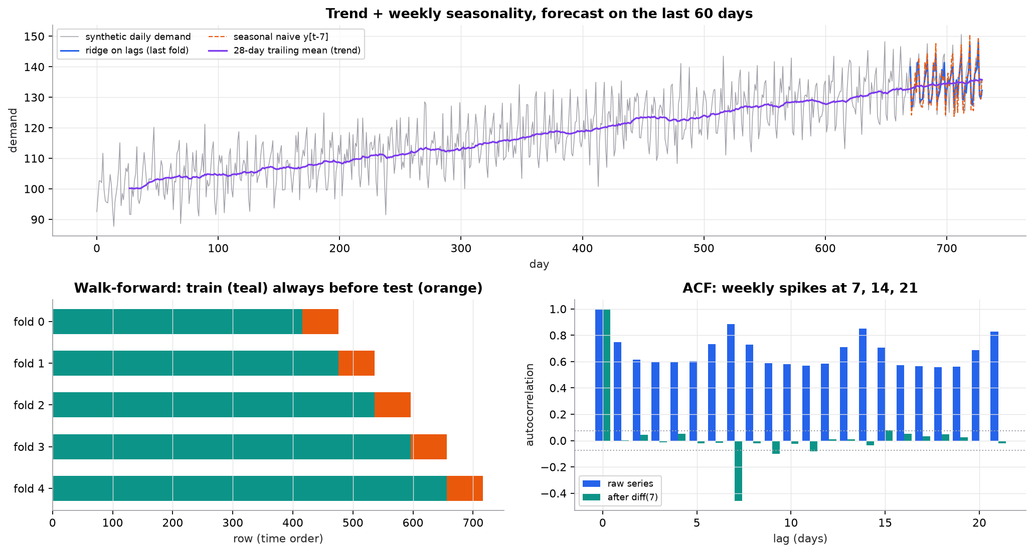
Synthetic daily series (trend 0.05 per day, weekly pattern, Gaussian noise). The raw ACF stays high at every lag because of the trend, with weekly spikes on top. Seasonal differencing removes both; the negative spike at lag 7 is the signature of differencing noise (see the math).

Try it (predict first, then run code/24-applied-ml/time_series.py):

Set the trend in make_series to 0. Predict what happens to the raw ACF at lags 1 to 6.
Remove lag 7 from lag_features (use lags=(1, 14)). Predict whether ridge still beats seasonal naive.
Raise the noise from 4 to 12. Predict which baseline's MAE grows more, and whether ridge's lead over seasonal naive grows or shrinks.
Change the leaky centered window to strictly trailing (y[t - 3:t]). Predict the walk-forward MAE.

3. The math

Symbols

Symbol	Meaning	Shape
$y_t$	value at time $t$	scalar; series is $[T]$
$\bar y$	mean of the series	scalar
$r_k$	sample autocorrelation at lag $k$	scalar
$m$	seasonal period (7 for daily data with a weekly pattern)	scalar
$\hat y_t$	forecast of $y_t$	scalar
$h$	forecast horizon (steps ahead)	scalar
$x_t$	feature row for time $t$ , built only from $y_{s}$ with $s < t$	$[p]$

Differencing and autocorrelation

\nabla y_t = y_t - y_{t-1}, \qquad \nabla_m y_t = y_t - y_{t-m}

r_k = \frac{\sum_{t=k+1}^{T} (y_t - \bar y)(y_{t-k} - \bar y)}{\sum_{t=1}^{T} (y_t - \bar y)^2}

For white noise, $r_k$ for $k \ge 1$ is about 0 with standard error about $1/\sqrt{T}$ , so bars outside $\pm 2/\sqrt{T}$ are worth a look (the dotted lines in the figure). If $y$ is white noise with variance $\sigma^2$ , then $\nabla_m y_t = e_t - e_{t-m}$ has variance $2\sigma^2$ and covariance $-\sigma^2$ at lag $m$ , so its autocorrelation at lag $m$ is $-\sigma^2 / 2\sigma^2 = -0.5$ . That's the $-0.46$ spike in the figure: differencing is removing the seasonal pattern and slightly over-correcting the noise.

Baselines and metrics

\hat y_t^{\text{naive}} = y_{t-1}, \qquad \hat y_t^{\text{snaive}} = y_{t-m}

\text{MAE} = \frac{1}{n}\sum |y_t - \hat y_t|, \qquad \text{MAPE} = \frac{100}{n}\sum \left|\frac{y_t - \hat y_t}{y_t}\right|, \qquad \text{MASE} = \frac{\text{MAE}}{\frac{1}{T-m}\sum_{t=m+1}^{T} |y_t - y_{t-m}|}

MAPE is undefined at $y_t = 0$ and punishes over-forecasts on small values. MASE divides by the in-sample error of the seasonal-naive forecast, so MASE below 1 means "better than seasonal naive", on any scale.

Worked example: a tiny series

$y = [10, 12, 14, 13, 15, 17, 16]$ , $T = 7$ .

Differences: $12-10, 14-12, 13-14, 15-13, 17-15, 16-17 = [2, 2, -1, 2, 2, -1]$ . The upward trend becomes a series with a steady mean of $6/6 = 1$ .
Mean: $\bar y = 97/7 = 13.857$ . Deviations, written in sevenths ( $7y_t - 97$ ): $[-27, -13, 1, -6, 8, 22, 15]/7$ .
Denominator: $(27^2 + 13^2 + 1^2 + 6^2 + 8^2 + 22^2 + 15^2)/49 = (729 + 169 + 1 + 36 + 64 + 484 + 225)/49 = 1708/49$ .
Lag-1 numerator: pairs of neighbors: $(-13)(-27) + (1)(-13) + (-6)(1) + (8)(-6) + (22)(8) + (15)(22) = 351 - 13 - 6 - 48 + 176 + 330 = 790$ , over 49.
$r_1 = 790/1708 = 0.4625$ : a neighbor tells you a lot, mostly because of the trend.
Naive MAE (forecast each of $t = 1..6$ with the previous value): errors are the absolute differences, $2, 2, 1, 2, 2, 1$ , so MAE $= 10/6 = 1.667$ .
MAPE of forecasting 16 with 17: $|16 - 17|/16 = 6.25\%$ .

Worked example: walk-forward on the synthetic series

716 feature rows (the first 14 days are used up by the lag-14 feature). Five folds, each testing the next 60 rows after everything before it:

Forecast	Mean MAE over 5 folds
Naive, $y_{t-1}$	6.91
Seasonal naive, $y_{t-7}$	4.32
Ridge on $y_{t-1}, y_{t-7}, y_{t-14}$ , trailing 7-day mean	3.79

Ridge's MASE (against in-sample seasonal naive) is 0.842: about 16% less error than the seasonal-naive baseline. The noise standard deviation is 4, so the best possible MAE is about $4\sqrt{2/\pi} = 3.19$ . The model is close, and much of the remaining gap is the weekly pattern being estimated from noisy lags.

4. Implementation

Build it from scratch

Diagnostics. Differencing and the ACF are a few lines each.

python

def difference(y, lag=1):
    """y'_t = y_t - y_{t-lag}. Loses the first `lag` points."""
    y = np.asarray(y, dtype=float)
    return y[lag:] - y[:-lag]

def acf(y, max_lag):
    """Sample autocorrelation r_k = sum (y_t - m)(y_{t-k} - m) / sum (y_t - m)^2."""
    y = np.asarray(y, dtype=float) - np.mean(y)
    denom = np.sum(y**2)
    return np.array([np.sum(y[k:] * y[: len(y) - k]) / denom for k in range(max_lag + 1)])

Predict: for a pure linear trend $y_t = t$ with no noise, is $r_1$ close to 0, 0.5, or 1?

Lag features. Row $t$ only reads indices strictly less than $t$ . The slice y[t - window:t] excludes $t$ because Python slices are end-exclusive.

python

def lag_features(y, lags=(1, 7, 14), window=7):
    """Row t uses y[t-l] for each lag and the mean of y[t-window : t] (strictly before t)."""
    y = np.asarray(y, dtype=float)
    start = max(max(lags), window)
    rows = []
    for t in range(start, len(y)):
        rows.append([y[t - l] for l in lags] + [y[t - window:t].mean()])
    return np.array(rows), y[start:], start

Predict: if you forecast 3 days ahead instead of 1, which of these features are no longer available at forecast time?

The leak, on purpose. A centered 3-day mean contains $y_t$ itself and $y_{t+1}$ .

python

def leaky_features(y, lags=(1, 7, 14), window=7):
    """BUG on purpose: same as lag_features, but the rolling mean is CENTERED (y[t-1], y[t], y[t+1])."""
    y = np.asarray(y, dtype=float)
    start = max(max(lags), window)
    rows = []
    for t in range(start, len(y) - 1):
        rows.append([y[t - l] for l in lags] + [y[t - 1:t + 2].mean()])
    return np.array(rows), y[start:len(y) - 1]

Predict: the leaky feature lowers MAE from 3.81 to 3.14 in walk-forward. What would its MAE be in production, where $y_t$ and $y_{t+1}$ aren't known yet?

Walk-forward splits and MASE.

python

def walk_forward(n, n_splits=5, test_size=60):
    """Expanding window: fold k trains on everything before its test block."""
    for k in range(n_splits):
        test_start = n - (n_splits - k) * test_size
        yield np.arange(test_start), np.arange(test_start, test_start + test_size)

python

def mase(y, yhat, y_train, m=1):
    """MAE scaled by the in-sample MAE of the (seasonal) naive forecast with period m."""
    scale = np.mean(np.abs(difference(y_train, m)))
    return mae(y, yhat) / scale

Predict: with a forecast horizon of 7 days, how big a gap should you leave between the end of each training block and its test block, and why?

Use the library

sklearn.model_selection.TimeSeriesSplit(n_splits=5, test_size=60, gap=0) produces the same expanding folds; max_train_size turns them into a sliding window, and gap drops rows between train and test so features that look back don't overlap the test period.
statsmodels provides seasonal decomposition (seasonal_decompose, STL), the ADF and KPSS stationarity tests, plot_acf/plot_pacf, and ARIMA/SARIMAX and exponential smoothing (ETS).
pandas shift(k) builds lags and rolling(w).mean().shift(1) builds a trailing window safely: the shift(1) is what keeps today out.
For many related series (every store and product), gradient-boosted trees on lag and calendar features (LightGBM) are a strong, common default. Libraries such as Nixtla's statsforecast and mlforecast, sktime, and Darts package these patterns. Pretrained forecasting foundation models (TimesFM, Chronos, Moirai) exist; benchmark them against seasonal naive on your own data before trusting them.

Run it

From guide/:

bash

uv run code/24-applied-ml/time_series.py

Key output:

text

acf lag 1    = 0.4625
naive MAE on t=1..6 = 1.6667
ACF diff(7)  lags 1, 7, 14: 0.002, -0.458, -0.035
mean first half = 108.95, second half = 127.34  (trend: not stationary)
  naive (y[t-1])           MAE = 6.91
  seasonal naive (y[t-7])  MAE = 4.32
  ridge on lags            MAE = 3.79
  ridge MASE (vs seasonal naive, m=7) = 0.842
  trailing features, walk-forward  MAE = 3.81  (honest)
  centered mean,     walk-forward  MAE = 3.14  (looks better: it peeks at y[t])

5. Engineering

Horizon decides features. A forecast for 14 days ahead can only use lags of 14 or more (or forecasts of the intermediate days). Decide the horizon first. Strategies: recursive (predict one step, feed it back; simple, errors compound), direct (one model per horizon; no compounding, more models), multi-output (one model emits all horizons).

Calendar and exogenous features. Day of week, month, holidays, promotions, price, and weather often matter more than deep lag structures. Exogenous features must also be known at forecast time: you'll know next week's planned promotion, but not next week's weather, only a forecast of it.

Expanding or sliding window. Expanding uses all history and suits stable processes. Sliding (fixed length) adapts when the world changes, such as after a pricing change or a pandemic.

Many series. One global model across thousands of related series (with series ID features) usually beats thousands of tiny local models, and handles new series better.

Uncertainty. Production forecasts feed decisions (stock levels, staffing), so give intervals: quantile regression, quantile loss in gradient boosting, or conformal prediction on walk-forward residuals.

Monitoring. Track error per horizon against the seasonal-naive baseline over time. Retrain on a schedule; when the error jumps, look for structural breaks such as new products or holidays the model never saw.

Watch out
Failure modes. Shuffled K-fold or a random train/test split. Centered or "full history" rolling features. Scaling or imputing with statistics computed over the whole series (including the future). Target alignment off by one, so $y_t$ appears among its own features. Reporting only MAPE on a series with values near zero. Not comparing with seasonal naive.

Common mistakes

df["roll7"] = df["y"].rolling(7).mean() without .shift(1): today's value is in today's feature.
Fitting trees on a trending series and expecting extrapolation beyond the training range.
Choosing lags from an ACF computed on the whole series, test period included (minor, but still lookahead).
Evaluating 1-step-ahead accuracy when the business needs 7-day-ahead forecasts.
Forward-filling missing values across long gaps, which invents flat stretches.

6. Knowledge check

Quiz: Time series

Question 1 of 10

Multiple choiceeasy

Why is a random train/test split invalid for time-series forecasting?

Practice exercise. Weekly sales for 8 weeks are $[20, 22, 21, 23, 25, 24, 26, 28]$ . You forecast weeks 5 to 8 using the naive method (last week's value). Compute the MAE and the MAPE.

Solution

Forecasts for weeks 5 to 8 are weeks 4 to 7: $23, 25, 24, 26$ . Actuals: $25, 24, 26, 28$ .

Absolute errors: $|25-23| = 2$ , $|24-25| = 1$ , $|26-24| = 2$ , $|28-26| = 2$ . MAE $= 7/4 = 1.75$ .

Percentage errors: $2/25 = 8.0\%$ , $1/24 = 4.17\%$ , $2/26 = 7.69\%$ , $2/28 = 7.14\%$ . MAPE $= (8.0 + 4.17 + 7.69 + 7.14)/4 = 27.0/4 = 6.75\%$ .

Implementation challenge. Add a recursive_forecast(model, history, h) that forecasts $h = 7$ days ahead from the end of the training data by predicting one day, appending the prediction to the history, and rebuilding features. Compare its 7-day MAE with seasonal naive on the last fold.

Solution

python

def recursive_forecast(model, history, h, lags=(1, 7, 14), window=7):
    hist = list(history)
    out = []
    for _ in range(h):
        t = len(hist)
        x = [hist[t - l] for l in lags] + [np.mean(hist[t - window:t])]
        yhat = float(model.predict([x])[0])
        out.append(yhat)
        hist.append(yhat)   # the forecast becomes "history" for the next step
    return np.array(out)

Fit ridge on the last fold's training rows, call it with history = y[:start + tr_last[-1] + 1], and compare with y[t-7] for the same 7 days. The lag-7 and lag-14 features are still real values for all 7 steps, while lag 1 and the rolling mean increasingly use forecasts. Expect the error to grow with the step and to land near seasonal naive by day 7. Averaging over many forecast origins (not one) is needed before concluding anything.

Summary

A time series is trend plus seasonality plus noise; differencing ( $\nabla$ , $\nabla_m$ ) removes trend and seasonality to approach stationarity.
The ACF shows which lags carry information; weekly data spikes at 7, 14, 21.
Lag and trailing-window features turn forecasting into regression, as long as row $t$ uses only the past.
Validate with walk-forward splits (TimeSeriesSplit), never shuffled K-fold.
Always report the naive and seasonal-naive baselines; MASE below 1 means you beat seasonal naive.

Next: Anomaly detection

Parts of this lesson are adapted from AI Engineering from Scratch by Rohit Ghumare (MIT license, notice): Time Series Fundamentals.

Interview angle

How would you split time-series data for validation, and why not use K-fold?

I'd use walk-forward validation: train on everything up to a cutoff, test on the next block, move the cutoff forward, and repeat, which is what scikit-learn's TimeSeriesSplit does. Each fold mimics production, where you only ever have the past. Shuffled K-fold puts future rows in the training set, so the model can interpolate between Friday and Sunday to predict Saturday, and lag features of test rows overlap training targets. The score comes out optimistic and the model ranking can be wrong. Choices to make: an expanding window if old data still applies, a sliding window if the process drifts. Make the test block length match the business horizon, say 7 or 28 days. Add a gap between train and test when features look back further than one step. Report the mean and the spread across folds, and compare every fold with the seasonal-naive baseline.

Classical models like ARIMA or ETS, or gradient boosting on lag features: how do you choose?

It depends on how many series you have, how long they are, and what drives them. For a few long, regular series with clear trend and seasonality, ARIMA or exponential smoothing are fast, give intervals, and are hard to beat. They model each series separately and handle external drivers only in limited ways (SARIMAX). For thousands of related series with promotions, prices, and holidays, one global gradient-boosting model on lag, rolling, and calendar features usually wins. It shares patterns across series and handles new ones. It does need care: features that only use the past, a differenced or trend-adjusted target because trees can't extrapolate, and recursive or direct strategies for multi-step horizons. Either way I'd start with seasonal naive, then pick by walk-forward MASE at the horizon the business uses. In the course's synthetic example, ridge on lags got MASE 0.84 against seasonal naive.

Your demand model had 3% MAPE in backtesting and 12% in production. What do you check?

First, lookahead in the backtest. Check every feature for a rolling window without a shift, a centered mean, an aggregate over the full history, or scaling fit on all data. In the course's example a centered 3-day mean cut MAE from 3.81 to 3.14 in a proper walk-forward split, and production can't compute it. Second, feature availability. Did the backtest use actual weather, promotions, or yesterday's sales when production only has forecasts, or data that arrives a day late? Third, horizon mismatch. Was the backtest one step ahead while production forecasts a week out? Fourth, the split itself. A random split instead of time-ordered folds inflates scores. Then real change: a structural break, new products, a holiday missing from training, or a data pipeline bug. I'd replay production inputs through the backtest code to see which difference closes the gap.

Your forecast has MAE 3.8 on a series whose seasonal-naive MAE is 4.5. What is its MASE, and is the model worth shipping?

MASE is the model's MAE divided by the seasonal-naive MAE, so 3.8 divided by 4.5 is about 0.84. The model makes about 16% less absolute error than "same day last week". Whether that's worth shipping depends on three checks. First, is the gain consistent? Look at MASE per walk-forward fold, and at the right horizon. A 16% average driven by one fold isn't reliable. Second, what is the error worth? If the forecast sets inventory, translate the error into stockouts and overstock costs, and compare that with the cost of running and monitoring a model. Third, is the denominator right? Strictly, MASE scales by the in-sample seasonal-naive error, and MASE below 1 means you beat that benchmark. I'd also check that the improvement survives the noise floor. With Gaussian noise of standard deviation 4, no model can get MAE much below about 3.2.