Module 24: Applied ML in practice 45 min10 min quick readClassical ML
Imbalanced data
Evaluate a classifier on rare positives with precision, recall, F1, MCC, and AUPRC, build SMOTE and class weights from scratch, and see that resampling mostly moves the threshold.
Before this: Classification metrics and thresholds, Logistic regression
Quick read: the intuition, interactive visualization, summary, and interview questions. The math, implementation, engineering, and knowledge-check sections are hidden.
Mental model. A smoke alarm in a kitchen almost never sees a real fire. An alarm that never rings is "right" 99.9% of the time and worthless. Handling imbalance means two things: score the alarm on the fires it catches and the false alarms it raises, and then decide deliberately how sensitive to set it. Most "fixes" for imbalance turn out to be different ways of turning that sensitivity knob.
You will learn to
- Explain why accuracy fails on rare positives and compute precision, recall, F1, MCC, and average precision (AUPRC) from a confusion matrix.
- Build random oversampling, random undersampling, SMOTE, and balanced class weights from scratch.
- Show that resampling and class weights mostly shift the decision threshold, and convert a threshold between the weighted and unweighted models.
- Tune a threshold on a validation set and keep resampling inside the training data only.
- Choose a strategy for a given imbalance ratio, data size, and cost of errors.
Why it matters. Fraud, disease screening, churn, defects, and intrusion detection all have rare positives, and they are the problems where mistakes cost the most. "My model gets 99% accuracy" is a red flag in an interview and in production. Knowing what each fix does, and what it does not do, separates a careful engineer from someone reaching for SMOTE by reflex.
1. Intuition
Take 800 transactions where 34 are fraud. A model that says "not fraud" every time gets accuracy and catches nothing. Accuracy rewards the majority class because every row counts equally, and almost every row is negative.
So first, change the scoreboard. Ask two questions about the positive class:
- Precision: of the transactions we flagged, how many were fraud?
- Recall: of the fraud that happened, how much did we flag?
F1 combines the two. MCC uses all four cells of the confusion matrix and is 0 for any constant predictor. Average precision (the area under the precision-recall curve, AUPRC) scores the whole ranking without picking a threshold, and a random ranking scores the positive rate, not 0.5.
Second, decide how the model should treat the rare class. There are three families of fixes:
- Change the data. Duplicate positives (random oversampling), throw away negatives (random undersampling), or invent new positives between real ones (SMOTE).
- Change the loss. Give each positive a bigger weight, so a missed fraud costs as much as roughly 19 false alarms.
- Change the threshold. Keep the model as it is and flag anything with predicted probability above, say, 0.24 instead of 0.5.
Here is the part that surprises people. For a model like logistic regression, all three mostly do the same thing: they move the decision boundary toward the majority class. They change where you operate on the precision-recall trade-off. They barely change how well the model ranks positives above negatives. If you tune the threshold properly, the plain model often does as well as any rebalanced one.
2. Visualization
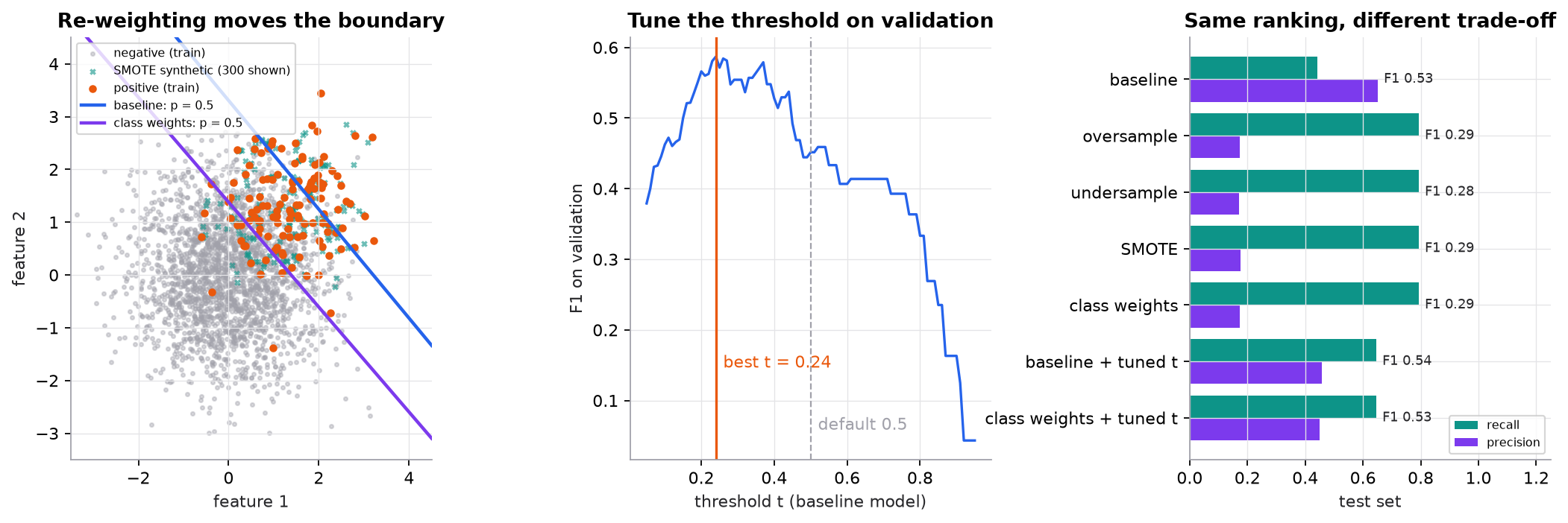
Synthetic data: two overlapping 2D Gaussian blobs, 4,000 points, 5% positive, split 2,400 / 800 / 800 into train, validation, and test. Left: class weights push the 0.5 boundary into the negatives. Middle: the best F1 threshold for the unweighted model is 0.24. Right: every rebalancing method lands on almost the same operating point, and tuning the threshold of either the plain or the weighted model reaches the same better one.
Try it (run the script, predict first, then check):
- Change
rng.normal(1.3, 0.8, ...)torng.normal(2.5, 0.8, ...)so the classes barely overlap. Predict whether the gap between "baseline" and "class weights" in F1 grows or shrinks. - Change the split to
n_neg=3960, n_pos=40(1% positive). Predict what happens to the AUPRC of a random scorer and to the stability of the tuned threshold. - Tune the threshold on the test set instead of validation by swapping
y_va, X_vafory_te, X_tein the tuning loop. Predict whether the reported test F1 goes up, and explain why that number is now untrustworthy. - In
smote, setk=1. Predict how the teal synthetic points change in the left panel.
3. The math
Symbols
| Symbol | Meaning | Shape |
|---|---|---|
| TP, FP, FN, TN | true positives, false positives, false negatives, true negatives | scalars |
| number of training rows; rows in class | scalars | |
| number of classes | scalar | |
| loss weight for every row of class | scalar per class | |
| positive rate (prior) in the training data | scalar | |
| predicted probability of the positive class | scalar per row | |
| decision threshold: predict positive if | scalar | |
| a minority point and one of its nearest minority neighbors | ||
| random interpolation factor in SMOTE, uniform on | scalar |
Metrics
MCC runs from to and is 0 for random or constant predictions. Average precision ranks rows by score and averages the precision at each true positive's rank:
where is the number of positives and if the row at rank is positive. A random ranking has expected AP equal to the positive rate.
Balanced class weights and weighted loss
Each class then carries the same total weight, .
SMOTE
Weights move the intercept, so they move the threshold
Up-weighting positives by the ratio is like training on data where positives are times more common. For a logistic model this mostly adds to the logit, so it multiplies the predicted odds by about . To convert a weighted model's probability back to the real-world scale (prior correction):
For balanced weights, . The same formula maps a threshold on the weighted model to the equivalent threshold on the unweighted one. It is approximate here because the two classes have different spreads, so the true log-odds are not exactly linear.
Worked example (numbers match the script)
1. The accuracy trap. The test set has 34 positives in 800 rows. Always predicting negative gives , , . Accuracy . Recall , so F1 . The MCC numerator is , so MCC .
2. Class weights. Training has rows, positives, negatives, .
- , so one positive counts as 18.83 negatives.
- Check: and . Each class carries half the total weight.
3. One SMOTE point. , neighbor , . The difference is ; times 0.4 gives ; added to gives .
4. Metrics for the weighted model at t = 0.5. On test: , , , .
- Precision
- Recall
- F1
- MCC numerator
- MCC denominator
- MCC
- Accuracy , lower than the useless model's 0.958, yet this model catches 79% of fraud.
5. Same model, different threshold. Tuned on validation, the best F1 threshold is 0.86 for the weighted model and 0.24 for the unweighted one. Convert 0.86 to the unweighted scale:
- Weighted odds
- Divide by :
- Back to a probability:
That is the 0.24 found independently for the unweighted model. Both tuned models land at test recall 0.647 and F1 about 0.53, and their AUPRC is 0.548 versus 0.551. The weights moved the threshold; they did not make a better ranker.
6. Prior correction. A weighted model says . With , : odds , divided by 18.83 gives , so . A "60% fraud" score from the weighted model means about 7% fraud in reality.
4. Implementation
The full script is code/24-applied-ml/imbalanced_data.py. It uses only NumPy for the from-scratch parts and checks itself against scikit-learn.
Build it from scratch
Metrics. Count the four confusion cells once, then derive everything from them. The if ... else 0.0 guards handle the cases where nothing is predicted positive, which is common with rare classes.
def metrics(y, pred):
    tp, fp, fn, tn = confusion(y, pred)
    precision = tp / (tp + fp) if tp + fp else 0.0
    recall = tp / (tp + fn) if tp + fn else 0.0
    f1 = 2 * precision * recall / (precision + recall) if precision + recall else 0.0
    denom = np.sqrt(float((tp + fp) * (tp + fn) * (tn + fp) * (tn + fn)))
    mcc = (tp * tn - fp * fn) / denom if denom else 0.0
    return {"precision": precision, "recall": recall, "f1": f1, "mcc": mcc}
Predict: for a model that flags every row as positive, which of precision, recall, F1, and MCC is 1, which is the positive rate, and which is 0?
Average precision. Sort by score, walk down the ranking, and record the precision each time you hit a positive. No threshold is involved; only the order matters.
def average_precision(y, scores):
    order = np.argsort(-scores)             # rank by score, highest first
    hits = y[order]
    precision_at_k = np.cumsum(hits) / np.arange(1, len(hits) + 1)
    return float(np.sum(precision_at_k * hits) / hits.sum())  # mean precision at each true positive
Predict: if you replace scores with 2 * scores + 1, does AP change?
Random over- and undersampling. Oversampling repeats positives until the classes match; undersampling keeps every positive and a random sample of negatives of the same size.
def random_oversample(X, y, rng):
    pos = np.where(y == 1)[0]
    extra = rng.choice(pos, size=int((y == 0).sum()) - len(pos), replace=True)  # duplicates
    keep = np.concatenate([np.arange(len(y)), extra])
    return X[keep], y[keep]

def random_undersample(X, y, rng):
    pos = np.where(y == 1)[0]
    neg = rng.choice(np.where(y == 0)[0], size=len(pos), replace=False)  # discards most negatives
    keep = np.concatenate([pos, neg])
    return X[keep], y[keep]
Predict: with 2,279 negatives and 121 positives, how many rows does each function return, and how many distinct positive rows does the oversampled set contain?
SMOTE. For each new point: pick a real minority point, pick one of its nearest minority neighbors, and place the new point at a random spot on the segment between them. Distances are computed among minority points only.
def smote(X_min, n_new, k, rng):
    d = np.linalg.norm(X_min[:, None, :] - X_min[None, :, :], axis=2)  # [m, m] pairwise distances
    np.fill_diagonal(d, np.inf)                                        # a point is not its own neighbor
    neighbors = np.argsort(d, axis=1)[:, :k]                           # [m, k] k nearest minority points
    base = rng.integers(0, len(X_min), size=n_new)                     # which real point to start from
    pick = neighbors[base, rng.integers(0, k, size=n_new)]             # one of its neighbors
    t = rng.random((n_new, 1))                                         # position along the segment
    return X_min[base] + t * (X_min[pick] - X_min[base])
Predict: a lone positive sits deep inside the negative cloud. Where do the synthetic points that start from it end up, and why is that a problem?
Weighted logistic regression. Plain gradient descent on cross-entropy, except each row's error is multiplied by its weight before it enters the gradient. Dividing by the total weight keeps the step size comparable to the unweighted version.
def fit_logreg(X, y, sample_weight=None, lr=0.5, epochs=2000):
    w_s = np.ones(len(y)) if sample_weight is None else sample_weight
    w, b = np.zeros(X.shape[1]), 0.0
    for _ in range(epochs):
        err = (sigmoid(X @ w + b) - y) * w_s           # each row's gradient scaled by its weight
        w -= lr * (X.T @ err) / w_s.sum()
        b -= lr * err.sum() / w_s.sum()
    return w, b

def balanced_weights(y):
    n, counts = len(y), np.bincount(y.astype(int))     # same rule as sklearn class_weight="balanced"
    per_class = n / (len(counts) * counts)
    return per_class[y.astype(int)], per_class
Predict: weighting every positive by 18.83 and oversampling every positive 18.83 times give the same loss in expectation. Which one is cheaper to train?
Threshold tuning. Sweep a grid of thresholds on the validation set and keep the one with the best F1. Swap F1 for expected cost or a recall floor when the business has one.
def best_threshold(y, probs):
    grid = np.round(np.arange(0.05, 0.96, 0.01), 2)
    f1s = np.array([metrics(y, (probs >= t).astype(int))["f1"] for t in grid])
    return float(grid[f1s.argmax()]), grid, f1s
Predict: the validation set has only 45 positives. If you rerun with a different seed, how much do you expect the chosen threshold to move?
Use the library
from sklearn.linear_model import LogisticRegression
from sklearn.metrics import average_precision_score, classification_report, matthews_corrcoef
from sklearn.model_selection import TunedThresholdClassifierCV   # scikit-learn >= 1.5
from imblearn.over_sampling import SMOTE                          # pip install imbalanced-learn
from imblearn.pipeline import Pipeline

# 1. Class weights: one argument.
weighted = LogisticRegression(class_weight="balanced").fit(X_train, y_train)

# 2. Threshold tuning with internal cross-validation (no hand-written loop, no test peeking).
tuned = TunedThresholdClassifierCV(LogisticRegression(), scoring="f1", cv=5).fit(X_train, y_train)
print(tuned.best_threshold_, average_precision_score(y_test, tuned.predict_proba(X_test)[:, 1]))

# 3. SMOTE inside a pipeline, so resampling only ever touches the training folds.
smote_model = Pipeline([("smote", SMOTE(k_neighbors=5, random_state=0)),
                        ("clf", LogisticRegression())]).fit(X_train, y_train)
print(classification_report(y_test, smote_model.predict(X_test), digits=3))
What the library adds: class_weight="balanced" computes exactly ; TunedThresholdClassifierCV tunes the cut-off with cross-validation and refits; imbalanced-learn's Pipeline applies samplers during fit only, never during predict, which is what keeps SMOTE from leaking into evaluation. Tree boosters have their own knob: scale_pos_weight in XGBoost and LightGBM, typically set near .
Run it
From guide/:
uv run code/24-applied-ml/imbalanced_data.pyKey output:
positives: train 121/2400, val 45/800, test 34/800  (synthetic)
always-negative on test: accuracy 0.958, recall 0.000, F1 0.000, MCC 0.000
class weights: n=2400, n_pos=121, w_neg=0.5265, w_pos=9.9174, ratio=18.83
best F1 threshold for baseline (tuned on validation): 0.24
best F1 threshold for class weights (tuned on validation): 0.86

strategy                 thresh   prec  recall     F1    MCC  AUPRC
baseline                   0.50  0.652   0.441  0.526  0.520  0.548
oversample                 0.50  0.174   0.794  0.286  0.320  0.551
undersample                0.50  0.172   0.794  0.283  0.317  0.540
SMOTE                      0.50  0.175   0.794  0.287  0.321  0.552
class weights              0.50  0.174   0.794  0.286  0.320  0.551
baseline + tuned t         0.24  0.458   0.647  0.537  0.521  0.548
class weights + tuned t    0.86  0.449   0.647  0.530  0.515  0.551
AUPRC of a random scorer = positive rate = 0.043
checks passed: matches sklearn class_weight='balanced' on 100.0% of test rows
Read the AUPRC column: every strategy ranks positives almost equally well (0.540 to 0.552). The F1 column differs because each strategy sits at a different operating point. On this data, the four rebalancing methods at threshold 0.5 overshoot toward recall, and tuning the threshold beats all of them.
5. Engineering
Start with the scoreboard. Pick the metric from the decision the model drives. Use a cost-weighted metric if you can price a false negative and a false positive (classification metrics shows how). Use recall at a fixed precision (or precision at a fixed alert budget) when a team can only review so many alerts a day. Report AUPRC for ranking quality and always state the positive rate next to it, since that is its random baseline.
Default recipe. A stratified split, a strong model on the raw data, then tune the threshold on validation. Add class weights if the learner struggles to fit the minority class at all (common with gradient boosting on 1:1000 data, or with neural networks where most batches hold no positives). Reach for resampling when you need it for speed (undersampling huge negative sets) or when a specific model benefits; measure it rather than assuming.
Calibration. Resampling and class weights distort predicted probabilities toward 50%. That matters when probabilities are used as probabilities: risk scores, expected-cost decisions, pricing. Apply prior correction or recalibrate on untouched validation data (CalibratedClassifierCV). Research on clinical risk models (van den Goorbergh et al., JAMIA 2022) found imbalance corrections made logistic models badly miscalibrated without improving discrimination.
Undersampling at scale. With billions of negatives (ad clicks, search logs), downsampling negatives is standard because it cuts training cost. Keep the sampling rate and correct predictions afterwards with the same odds formula, or weight the kept negatives by the inverse sampling rate.
SMOTE limits. It interpolates in feature space, so it needs meaningful distances: scale features first, and it does not suit raw categorical data (use SMOTENC or SMOTEN), text, or images. It amplifies label noise and outliers, and it can paint synthetic positives into negative regions. Variants such as Borderline-SMOTE and ADASYN change which points seed new samples, not the core limitation.
Data size. With only a few dozen positives, every estimate is noisy: the tuned threshold, F1, even AUPRC. Use repeated stratified cross-validation, report intervals, and spend effort on getting more labeled positives, which usually beats any resampling trick.
Monitoring. The positive rate drifts (fraud waves, seasonal disease). Precision at a fixed threshold drifts with it. Track the live positive rate and alert volume, and revisit the threshold when either moves.
Common mistakes
- Resampling before the train/test split, or before cross-validation folds are made. Synthetic or duplicated positives leak into evaluation and inflate every metric.
- Evaluating on a rebalanced test set. The test set must keep the real class ratio, or precision is meaningless.
- Tuning the threshold on the test set, then reporting test performance as if it were unseen.
- Reporting accuracy or ROC AUC alone on a 1% positive problem, or AUPRC without the positive rate.
- Treating a class-weighted model's output as a calibrated probability.
- Applying SMOTE to one-hot categorical columns and producing "0.37 of a country".
6. Knowledge check
Quiz: Imbalanced data
A fraud dataset has 99.9% legitimate transactions and 0.1% fraud. A model predicts "legitimate" for every transaction. What is its accuracy?
Practice exercise. A fraud model reviewed on 10,000 transactions (50 fraud) gives , , . Compute accuracy, precision, recall, F1, and MCC. Then compute the balanced class weights for the training set this came from if it had the same ratio.
Solution
.
- Accuracy
- Precision
- Recall
- F1
- MCC numerator
- MCC denominator
- MCC
Weights with , , : , , ratio . Accuracy (0.983) is below the always-negative baseline (0.995), while the model catches 80% of fraud.
Implementation challenge. Add a cost-based threshold to the script: given and , pick the validation threshold that minimizes for the baseline model, and report the test cost next to the F1-tuned threshold's cost. Then check it against the theoretical cut-off for a calibrated model, .
Solution
def best_cost_threshold(y, probs, c_fn=50, c_fp=1):
    grid = np.round(np.arange(0.01, 0.96, 0.01), 2)
    costs = []
    for t in grid:
        tp, fp, fn, tn = confusion(y, (probs >= t).astype(int))
        costs.append(c_fn * fn + c_fp * fp)
    return float(grid[int(np.argmin(costs))])
The theoretical cut-off is : flag whenever the chance of fraud exceeds about 2%, because a miss costs 50 times a false alarm. On the script's validation set the sweep picks 0.02, matching theory, because unweighted logistic regression is reasonably calibrated. Expect a much lower threshold and higher recall than the F1-tuned 0.24, at the price of many more alerts. If you try the same with the class-weighted model, the cost-optimal threshold moves far higher, because its probabilities are inflated by about 18.83 in odds.
Summary
- Accuracy is dominated by the majority class; use precision, recall, F1, MCC, cost, and AUPRC, and quote AUPRC with the positive rate.
- Oversampling, undersampling, SMOTE, and class weights all push the boundary toward the majority class; for a linear model they mainly change the operating point, not the ranking.
- Class weights of multiply the predicted odds by about ; divide by that ratio to recover real-world probabilities or to translate thresholds.
- Tune the threshold on validation (or with
TunedThresholdClassifierCV) against the metric the business cares about. It is often the whole fix. - Resample only inside training folds, keep the test set at the true ratio, and recalibrate if anyone reads the scores as probabilities.
Next: Hyperparameter tuning
Related: Classification metrics and thresholds · Logistic regression · Anomaly detection · Feature engineering
Parts of this lesson are adapted from AI Engineering from Scratch by Rohit Ghumare (MIT license, notice): Handling Imbalanced Data.
Interview angle
Your fraud model has 99% accuracy. Why might that be meaningless, and what would you report instead?
If fraud is 1% of transactions, a model that never flags anything also scores 99%, so accuracy alone says nothing about the class we care about. I'd report the positive rate first, then precision and recall at the operating threshold, because those map to business questions: what fraction of alerts are real, and what fraction of fraud we catch. F1 or MCC give a single summary at that threshold; MCC is nice because any constant predictor scores 0. To judge the ranking independent of threshold I'd use average precision, the area under the precision-recall curve, and state that a random ranking scores the positive rate, here 0.01, not 0.5. ROC AUC can look strong on very rare positives because the false positive rate divides by a huge negative count. Finally, if analysts review alerts, I'd report recall at the alert volume they can handle, and the expected cost if we can price misses and false alarms.
Class weights, SMOTE, undersampling, or threshold tuning: how do you choose?
I'd start with no rebalancing plus a threshold tuned on validation, because for a model like logistic regression the other fixes mostly move the decision boundary toward the majority class, which is what a lower threshold does. In the course's synthetic example, balanced weights multiplied the odds by 18.83, and the best weighted threshold, 0.86, mapped back to 0.246 on the plain model, which had independently picked 0.24; ranking quality was the same. Class weights earn their place when the learner barely fits the minority class, like boosting at 1:1000 or neural nets with few positives per batch. Undersampling is for cost: billions of negatives are wasteful to train on, but you must correct the probabilities afterwards. SMOTE needs meaningful distances and enough positives for neighbors; it suits continuous features and is measured, not assumed. Any choice also distorts calibration, so I'd recalibrate if scores are used as probabilities.
A teammate reports F1 jumped from 0.45 to 0.80 after adding SMOTE. What do you check?
A jump that large from resampling alone is suspicious, so I'd look for leakage first. Was SMOTE applied before the train/test split or before cross-validation folds were made? Then synthetic points interpolated from test positives sit in training, and near-copies of training positives sit in test, which inflates everything. The fix is to resample inside each training fold, for example with imbalanced-learn's Pipeline. Second, is the test set still at the real class ratio? If it was rebalanced, precision is computed on a fake 50/50 world and will be far higher than in production. Third, was the threshold tuned on the test set? Fourth, compare AUPRC before and after: if ranking quality is unchanged, the "gain" is only a threshold shift that tuning the original model would match. Finally, check variance across seeds, since with few positives F1 can swing a lot by chance.
You trained with class_weight balanced at a 1 to 19 ratio. The model outputs 0.6 for a case. What is the real fraud probability?
Balanced weights make each class carry equal total weight, which acts like training on a world where positives are about 19 times more common than they are. For logistic regression that mostly adds ln 19 to the logit, so the predicted odds are inflated by about 19. To undo it, convert to odds, divide by the ratio, and convert back. The model's 0.6 is odds of 0.6 over 0.4, which is 1.5. Dividing by 19 gives about 0.079. Converting back, 0.079 over 1.079 is about 0.073, so roughly 7%, not 60%. The same arithmetic translates thresholds: a weighted threshold of 0.86 is odds 6.14, divided by 19 is 0.32, which is a probability of about 0.24 on the unweighted scale. This is approximate, so for anything that consumes probabilities I'd recalibrate on untouched validation data with Platt scaling or isotonic regression.