Module 24: Applied ML in practice 40 min10 min quick readClassical ML
Anomaly detection
Find rare, unusual points without labels using robust z-scores, IQR fences, k-NN distance, LOF, and isolation forests, then set thresholds from an alert budget and evaluate with the few labels you have.
Before this: Probability and statistics, K-nearest neighbors
Quick read: the intuition, interactive visualization, summary, and interview questions. The math, implementation, engineering, and knowledge-check sections are hidden.
Mental model. An anomaly detector learns what "normal" looks like and scores how far each point is from it. Statistical rules measure distance from the center in units of spread. Neighbor methods ask how lonely a point is. An isolation forest asks how few random cuts it takes to fence a point off on its own. None of them knows what you care about, so a human-sized alert budget and a few labels decide the threshold.
You will learn to
- Explain why anomaly detection is usually unsupervised, and name point, contextual, and collective anomalies.
- Compute a z-score, a robust (MAD) z-score, and IQR fences by hand, and show how one outlier hides itself from the plain z-score.
- Score points by k-NN distance and LOF, and say when local density matters.
- Build an isolation forest and compute its score from path lengths with the normalizer.
- Set a threshold from an alert budget and evaluate with precision at k and AUPRC.
Why it matters. Fraud, intrusion, equipment failure, data-quality checks, and metric monitoring are all anomaly detection. Labels are scarce and new failure types keep appearing, so a supervised classifier alone misses exactly the cases you most want to catch. Interviewers use it to test whether you can reason about evaluation when you have almost no labels.
1. Intuition
Why unsupervised. Anomalies are rare (often under 1%), labeling them is slow, and tomorrow's anomaly may look nothing like yesterday's. So we model normal data and flag what doesn't fit. If you do have plenty of labels for a known pattern (chargebacks for a known fraud type), a supervised classifier on imbalanced data is better for that pattern. Production systems often run both.
Three kinds. A point anomaly is strange on its own (a USD 50,000 coffee purchase). A contextual anomaly is strange only in context (90°F is normal in July and alarming in January; see time series). A collective anomaly is a group of normal-looking points that is strange together (a burst of small logins from one IP).
Statistical rules. Measure distance from the center in units of spread: the z-score uses mean and standard deviation. The catch is that the outlier inflates both, so it can hide itself. The median and the median absolute deviation (MAD) barely move when one point goes wild, so the robust z-score keeps working. IQR fences (the box-plot rule) are another robust option.
Neighbors. In more than one dimension, a point can be normal on every feature and still sit in an empty region. Distance to the k-th nearest neighbor captures that. LOF (local outlier factor) compares a point's neighborhood density with its neighbors' densities, so a point near a tight cluster is judged against tight standards and a point in a diffuse cluster against loose ones.
Isolation. Pick a random feature and a random split value, and repeat. A point far from everyone gets separated in a few cuts. A point deep inside a cluster needs many. Average the number of cuts over many random trees: short paths mean anomalies. No distances, near-linear cost, works well in moderate dimensions.
2. Visualization
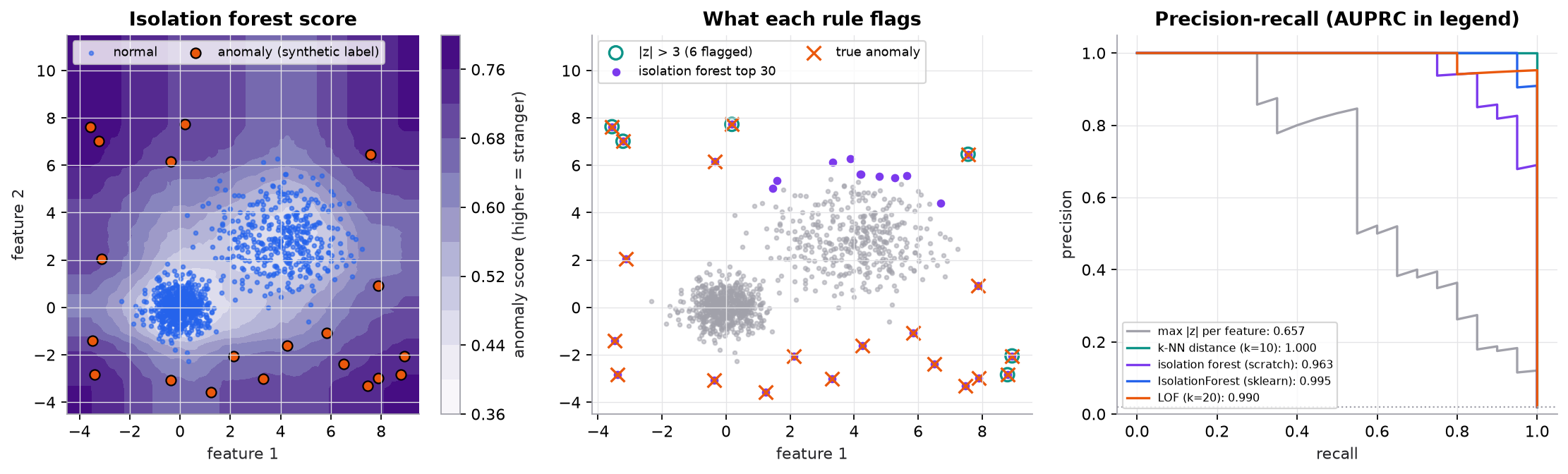
Synthetic data: 980 normal points in two Gaussian clusters with different spreads, plus 20 scattered anomalies (2%). Labels are used only to evaluate. The z-score rule catches only anomalies that are extreme on a single feature; anomalies in the gap between clusters are invisible to it.
Try it (predict first, then run code/24-applied-ml/anomaly_detection.py):
- Change
xin the worked example to contain two 50s. Predict whether the robust z-score still flags them. - Change the alert
budgetfrom 30 to 15. Predict precision and recall. - Shrink cluster
b's spread from 1.2 to 0.6. Predict whether k-NN distance or LOF benefits more. - In
isolation_forest, setn_trees=5. Predict whether AUPRC drops a little or a lot, and why.
3. The math
Symbols
| Symbol | Meaning | Shape |
|---|---|---|
| one feature over points | ||
| mean and standard deviation | scalars | |
| median | scalar | |
| median of | scalar | |
| 25th and 75th percentiles | scalars | |
| path length of a point in one isolation tree (number of edges to its leaf) | scalar | |
| subsample size per isolation tree (default 256) | scalar | |
| average path length of an unsuccessful search in a binary search tree of points | scalar | |
| isolation forest anomaly score | scalar in |
Statistical rules
The constant 0.6745 is the 75th percentile of the standard normal, so for Gaussian data the robust z-score matches the ordinary one. A common cutoff (Iglewicz and Hoaglin) is .
Isolation forest score
with (Euler's constant), , and . When a leaf still holds several points because the depth limit was reached, is added to its depth as an estimate of the unbuilt subtree. If then (anomaly); if then ; deeper than average gives (normal).
Worked example: one outlier masks itself
, .
- Mean: .
- Squared deviations: , , twice, , , . Sum .
- .
- . Below 3, so not flagged. The 50 inflated both the mean and the standard deviation.
- Robust: median . Absolute deviations ; sorted ; MAD .
- . Far above 3.5: flagged.
- IQR (linear interpolation): , , IQR . Fences . 50 is outside: flagged.
Worked example: isolation forest scores
With : .
- A point isolated in cuts: . Anomalous.
- : . Average.
- : . Normal.
In the script, the 20 anomalies average 5.25 cuts and the normal points average 11.98.
4. Implementation
Build it from scratch
Statistical rules. Three one-liners. The robust version swaps mean for median and standard deviation for MAD.
def z_scores(x):
    x = np.asarray(x, dtype=float)
    return (x - x.mean()) / x.std()

def robust_z(x):
    """Modified z-score: 0.6745 * (x - median) / MAD. 0.6745 makes it match z for Gaussian data."""
    x = np.asarray(x, dtype=float)
    med = np.median(x)
    mad = np.median(np.abs(x - med))
    return 0.6745 * (x - med) / mad

def iqr_fences(x, k=1.5):
    q1, q3 = np.percentile(x, [25, 75])
    return q1 - k * (q3 - q1), q3 + k * (q3 - q1)
Predict: what does robust_z do if more than half the values are identical? (Hint: what is the MAD?)
k-NN distance. Sort each row of the pairwise distance matrix and read the k-th entry. same=True skips the zero distance to itself.
def knn_score(X_ref, X, k=10, same=True):
    """Distance to the k-th nearest reference point. If same, skip the zero distance to itself."""
    d = np.sqrt(((X[:, None, :] - X_ref[None, :, :]) ** 2).sum(-1))
    d.sort(axis=1)
    return d[:, k] if same else d[:, k - 1]
Predict: the distance matrix is . At , is this approach still usable? What would you use instead?
The normalizer and one isolation tree. A random feature, a random split between its min and max, recurse until a point is alone or the depth limit is hit.
def c(n):
    """Average path length of an unsuccessful BST search over n points; normalizes depths."""
    if n <= 1:
        return 0.0
    if n == 2:
        return 1.0
    return 2 * (math.log(n - 1) + EULER) - 2 * (n - 1) / n

def build_tree(X, depth, max_depth, rng):
    """Split on a random feature at a random value until a point is alone or depth runs out."""
    if depth >= max_depth or len(X) <= 1:
        return {"size": len(X)}
    f = rng.integers(X.shape[1])
    lo, hi = X[:, f].min(), X[:, f].max()
    if lo == hi:
        return {"size": len(X)}
    v = rng.uniform(lo, hi)
    left = X[:, f] < v
    return {"f": f, "v": v,
            "l": build_tree(X[left], depth + 1, max_depth, rng),
            "r": build_tree(X[~left], depth + 1, max_depth, rng)}
Predict: why is it fine to stop at depth 8 for instead of growing the tree fully?
Path length and the forest. Each tree sees a random subsample of 256 points; the score averages path lengths over trees.
def path_length(x, node, depth=0):
    """Edges from root to the leaf containing x, plus c(size) for the unbuilt subtree below a leaf."""
    if "size" in node:
        return depth + c(node["size"])
    child = node["l"] if x[node["f"]] < node["v"] else node["r"]
    return path_length(x, child, depth + 1)

def isolation_forest(X, n_trees=100, sample=256, seed=0):
    """Returns s(x) = 2^(-E[h(x)] / c(sample)) for every row: near 1 = anomaly, about 0.5 or less = normal."""
    rng = np.random.default_rng(seed)
    psi = min(sample, len(X))
    max_depth = math.ceil(math.log2(psi))
    trees = [build_tree(X[rng.choice(len(X), psi, replace=False)], 0, max_depth, rng) for _ in range(n_trees)]
    mean_h = np.array([np.mean([path_length(x, t) for t in trees]) for x in X])
    return 2 ** (-mean_h / c(psi)), mean_h
Predict: subsampling 256 of 1,000 points per tree makes each tree see fewer anomalies. Why does that help rather than hurt? (Think about "masking" by clumps of anomalies.)
Use the library
from sklearn.ensemble import IsolationForest
from sklearn.neighbors import LocalOutlierFactor

iso = IsolationForest(n_estimators=200, contamination="auto", random_state=0).fit(X_train)
scores = -iso.score_samples(X_new)            # higher = more anomalous
lof = LocalOutlierFactor(n_neighbors=20, novelty=True).fit(X_train)
lof_scores = -lof.score_samples(X_new)score_samplesreturns the negated paper score, so flip the sign.predictreturns for anomalies using a threshold set bycontamination; with"auto"the threshold is fixed at paper score 0.5.LocalOutlierFactorscores the training data by default; setnovelty=Trueto score new points.- Also in scikit-learn:
OneClassSVMandEllipticEnvelope(robust covariance, Mahalanobis distance). PyOD collects dozens of detectors behind one API. - For high-dimensional data (images, logs, embeddings), an autoencoder's reconstruction error is a common score: train on normal data, flag inputs it reconstructs badly. Distance in a pretrained embedding space is a simpler alternative worth trying first.
Run it
From guide/:
uv run code/24-applied-ml/anomaly_detection.pyKey output:
mean = 17.43, std = 13.35, z(50) = 2.44  -> NOT flagged at |z| > 3
median = 12, MAD = 1, robust z(50) = 25.63  -> flagged at |z| > 3.5
c(256) = 10.245
  max |z| per feature          AUPRC = 0.657   precision@20 = 0.55
  k-NN distance (k=10)         AUPRC = 1.000   precision@20 = 1.00
  isolation forest (scratch)   AUPRC = 0.963   precision@20 = 0.85
  IsolationForest (sklearn)    AUPRC = 0.995   precision@20 = 0.95
  LOF (k=20)                   AUPRC = 0.990   precision@20 = 0.95
  scratch IF mean path length: anomalies 5.25, normals 11.98
flag top 30: threshold s >= 0.610, caught 20 of 20 anomalies, precision = 0.67, recall = 1.00
The k-NN score is perfect here because this synthetic data was built to make the anomalies far from both clusters. Don't read it as a ranking of methods in general; on real data, compare detectors on your own labeled incidents.
5. Engineering
Thresholds come from capacity. A detector outputs a score, not a decision. Decide how many alerts a team can review per day (the alert budget), and flag that many top scores. contamination is the same idea expressed as a fraction. Revisit the threshold as volume changes.
Evaluation with few labels. Use whatever labels exist (past incidents, chargebacks, analyst verdicts) as a test set. Report precision at the alert budget and AUPRC (the random baseline is the anomaly rate, not 0.5). Run new detectors in shadow mode and have analysts label a sample of their top alerts. Labels gathered only from your current detector's alerts are biased toward what it already catches.
Features matter more than the algorithm. Scale features before distance methods (feature engineering). Encode context explicitly (hour of day, account age, rolling per-user baselines), which turns contextual anomalies into point anomalies. For time series, score the residual after removing trend and seasonality, not the raw value.
Cost. Isolation forest trains in roughly for trees and scores each point in , independent of training size. Exact k-NN and LOF need neighbor search over the training set; use approximate nearest-neighbor indexes at scale.
Drift and feedback. "Normal" moves. Retrain on recent data, but exclude confirmed anomalies, or the detector learns them as normal. Track alert volume and analyst precision over time.
Watch outFailure modes. A z-score on skewed or multimodal data. Training data contaminated with the anomalies you want to catch. Unscaled features dominating distances. Alert floods after a seasonal change. Many weak features in high dimensions, where all distances look alike. Treating "unusual" as "bad": many anomalies are benign (a big holiday purchase).
Common mistakes
- Using
predictwith the default threshold instead of choosing one from the alert budget. - Forgetting that
score_samplesis negated (higher means more normal). - Reporting ROC AUC alone at a 0.1% anomaly rate, where it looks excellent even with poor precision.
- Fitting LOF without
novelty=Trueand then calling it on new data. - Tuning hyperparameters on the same handful of labeled anomalies used to report performance.
6. Knowledge check
Quiz: Anomaly detection
Why is anomaly detection usually framed as an unsupervised problem rather than classification?
Practice exercise. Response times in milliseconds are . Compute the robust z-score of 400 and decide whether to flag it at 3.5. Then compute the IQR fences with .
Solution
Sorted: . Median . Absolute deviations (in the original order): ; sorted ; MAD .
. Flag it.
Quartiles (linear interpolation on 7 values): at position 1.5, between 99 and 100, so 99.5. at position 4.5, between 102 and 103, so 102.5. IQR . Fences . 400 is outside.
Implementation challenge. Add a "contextual" check for a daily metric: compute a robust z-score of each day against the same weekday over the previous 8 weeks, and flag days above 3.5.
Solution
def weekday_robust_z(y, weeks=8, period=7):
    y = np.asarray(y, dtype=float)
    out = np.full(len(y), np.nan)
    for t in range(weeks * period, len(y)):
        ref = y[t - period * np.arange(1, weeks + 1)]   # same weekday, previous weeks
        med = np.median(ref)
        mad = np.median(np.abs(ref - med)) or 1e-9
        out[t] = 0.6745 * (y[t] - med) / mad
    return out
The reference window uses only the past, so it can run live. Comparing with the same weekday removes the weekly pattern, so a normal Saturday peak isn't flagged while a Tuesday that looks like a Saturday is. Floor the MAD to avoid dividing by zero on flat metrics.
Summary
- Anomaly detection models normal data and scores deviation from it, because labeled anomalies are rare and new ones look different.
- Plain z-scores let outliers hide by inflating the mean and standard deviation; MAD-based robust z-scores and IQR fences don't.
- k-NN distance and LOF catch points that are normal on every feature but sit in empty regions; LOF adapts to local density.
- Isolation forests score by how few random cuts isolate a point: .
- Set thresholds from an alert budget; evaluate with precision at that budget and AUPRC on whatever labels you have.
Next: From text to vectors
Related: Imbalanced data · Time series · k-nearest neighbors · Density and mixture clustering
Parts of this lesson are adapted from AI Engineering from Scratch by Rohit Ghumare (MIT license, notice): Anomaly Detection.
Interview angle
How does an isolation forest detect anomalies, and why does it work?
It builds many random trees. Each tree takes a small subsample, usually 256 points, then repeatedly picks a random feature and a random split value between that feature's min and max, until points are isolated or a depth limit of about log2 of 256, so 8, is reached. Anomalies are few and far from the rest, so a random cut separates them early. Their average path length is short, while points deep in a cluster need many cuts. The score normalizes the average path length by c(256), about 10.2, the expected depth for random data: s equals 2 to the power of minus E[h] over c. That gives near 1 for anomalies, about 0.5 for average points, and below that for normal ones. In the course's synthetic data, anomalies averaged 5.3 cuts against 12.0 for normal points. It needs no distances, scales roughly linearly, and subsampling reduces masking by clumps of anomalies.
Isolation forest, LOF, or a robust z-score: how do you choose?
Start simple. For one metric at a time, such as latency or daily sales, a robust z-score with median and MAD, computed against the right context like the same weekday, is transparent, cheap, and easy to explain in an alert. It won't catch points that are only strange in combination. For tabular data with many features, isolation forest is a strong default. It's fast, needs little tuning, and handles mixed scales reasonably, though it still benefits from scaling. LOF compares each point with its neighbors' density, so it wins when clusters have very different spreads and an anomaly sits just outside a tight cluster. It needs neighbor search, which costs more at scale. For high-dimensional inputs like images or text, score distance or reconstruction error in an embedding space. Whatever I pick, I'd compare candidates on precision at the alert budget, using labeled past incidents.
Your z-score alerting rule missed a huge spike that was obvious on the dashboard. Why, and how do you fix it?
The spike probably hid itself. A z-score uses the mean and standard deviation, and if the window includes the spike, both get pulled toward it. In the course example, 50 among values around 12 gets a z of only 2.44, below a cutoff of 3. Other causes: the window is too long and the metric has a trend or weekly pattern, so the standard deviation is inflated by normal variation. Or the data is skewed and the Gaussian assumption doesn't hold. Fixes: use the median and MAD instead. The same 50 gets a robust z of 25.6. Compute the baseline only from past data, excluding the current point. Compare against the same context, such as the same hour or weekday, or score the residual after removing trend and seasonality. Then back-test the new rule on past incidents and on quiet periods, to check both missed spikes and false alarms.
You have 1 million events a day, analysts can review 200 alerts, and you have 50 labeled past incidents. How do you set up and evaluate the detector?
The budget fixes the operating point: flag the top 200 scores a day, which is 0.02% of events. So I care about precision at 200 and recall of real incidents within those 200, not overall accuracy or ROC AUC. With 50 labeled incidents, I'd keep them as a test set, possibly with a few for tuning, and score candidate detectors by how many incidents land in the top 200 on their day. AUPRC adds a threshold-free view; its random baseline is the incident rate. Labels are scarce and biased toward what was already caught, so I'd run the new detector in shadow mode for a few weeks. Analysts label a random sample of its top alerts, which estimates precision and surfaces new incident types. Then I'd monitor daily alert volume and analyst precision, and retrain on recent data with confirmed incidents removed so they don't become normal.